
Most option traders think that the calculations behind the formulas for option premiums and all the key Greek variables are too complicated to care about. And if you take a look at the equations from the Black-Scholes’ model, it is hard to argue that it isn’t complex. But over time, I’ve realized, as many traders have, that there are a lot of short-hand ways to think about how these various calculations come together that are much easier to grasp. Hopefully, this article will help make the various numbers much more relatable. At some level, you’ll hopefully be able to estimate option premiums.
How much does an option cost?
Options have three primary drivers for the amount of premium they are priced at: Implied Volatility, Time to Expiration, and Moneyness- how close the strike price is to the current price of the underlying security. Two other factors can also influence the cost of an option: interest rates and future dividends. Let’s look at each of the five to see how each gets to influence option premiums.
Traders often use a simplified shortcut to estimate the expected move and the rough premium of an at‑the‑money (ATM) option without diving into the full Black‑Scholes math.
The expected move over a given time period can be approximated as:
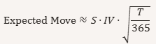
Where:
- S = current stock price
- IV = implied volatility (annualized, expressed as a decimal)
- T = days to expiration
This formula comes directly from the idea that volatility scales with the square root of time.
💰 Estimating ATM Option Premiums
For an At the Money (ATM) straddle (buying both the call and put at the same strike which very close to the current underlying price), the combined premium is often close to the expected move. That means:
ATM Straddle Premium ≈ 2⋅ATM Option Premium ≈ Expected Move
So, a single ATM option premium can be roughly estimated as:
ATM Option Premium ≈ Expected Move / 2
⚡ Quick Example
- Stock price (S) = $100
- Implied Volatility (IV) = 40% = 0.40
- Days to expiration (T) = 23 (23/365 ≈ 1/16) => Square root of 1/16 is 1/4, or 0.25
Expected Move≈100 x 0.40 x 1/4 = 10
So:
- ATM straddle ≈ $10.00 total premium
- Each ATM option ≈ $5.00
Usually, the math isn’t so easy to estimate option premiums that you can do it in your head like this example, but with a calculator, it can be pretty fast.
📘 Practical Notes
- This shortcut works best for near‑term ATM options.
- It’s less accurate for deep ITM/OTM strikes or very long‑dated expirations.
- Market makers adjust for skew, dividends, and rates, so actual premiums may differ.
- Still, this formula is widely used by traders to quickly gauge whether options look “rich” or “cheap” relative to implied volatility.
Options Out of the Money
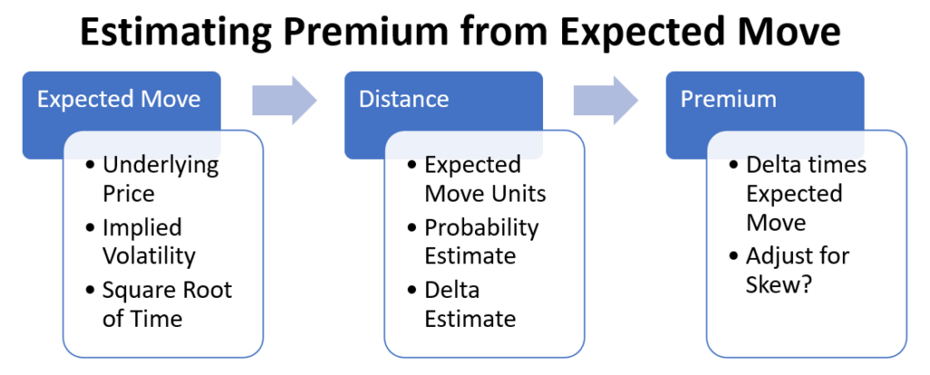
Most traders understand the expected move as a quick way to gauge how far a stock might travel over an option cycle, but the real magic happens when you use that same number to estimate the value of strikes across the entire chain. Once you know the expected move, you’re not just guessing at ATM pricing anymore—you’re holding a ruler that measures how “far” each strike sits in volatility terms. And once you can measure distance, you can estimate Delta, probability, and even a reasonable premium.
The first step is simply converting a strike into “expected‑move units.” If the stock is at 100 and the expected move is 8, then a 108 strike is exactly one expected move away. A 104 strike is half an expected move away. A 116 strike is two expected moves away. This framing is powerful because it strips away the noise of dollar amounts and replaces it with a standardized scale the market already uses implicitly.
Once you’ve expressed a strike in expected‑move units, you can start talking about probability in a way that feels natural. The expected move is essentially one standard deviation of price movement. So a strike that sits one expected move away corresponds to roughly a 16% chance of being reached. Two expected moves away? Now you’re down around 2–3%. Half an expected move? You’re in the 30% range. These aren’t exact numbers, but they’re close enough to give you a trader’s intuition for where the market thinks the action is.
This is where Delta enters the conversation. For out‑of‑the‑money options, Delta behaves very much like a probability proxy. A 30‑Delta call is telling you the market sees about a 30% chance of finishing in the money. A 16‑Delta call is signaling roughly a one‑standard‑deviation shot. A 5‑Delta call is living out in the tail. You don’t need to run Black‑Scholes to get these numbers—you can get surprisingly close just by knowing how many expected‑move units away the strike sits.
So now you’ve got a distance and a Delta. The next question is: can you turn that into a premium estimate? Absolutely. The same shortcut that tells you the ATM option is worth about half the expected move also tells you that an OTM option should be worth roughly its Delta multiplied by the expected move. If the expected move is 8 and the option has a 30 Delta, then a reasonable ballpark premium is 0.30 × 8 = 2.40. If the Delta is 16, you’re looking at something closer to 1.28. It’s not perfect, but it’s shockingly close to what you’ll see on a live chain.
This works because Delta isn’t just a directional sensitivity—it’s a probability‑weighted share of the expected move. The ATM option has a 50 Delta and captures about half the expected move. A 30‑Delta option captures about 30% of it. A 10‑Delta option captures about 10%. Market makers think in these terms constantly, and this shortcut gives you a window into their world without needing a volatility surface or a pricing model.
Another benefit of this approach is that it helps traders understand why OTM options get cheap so quickly. As you move farther out, the expected‑move distance grows, the probability shrinks, and the Delta collapses. That’s why a strike two expected moves away might only be worth a few pennies even when the expected move itself is large. You’re not paying for the size of the move—you’re paying for the probability of reaching it.
This framework also helps explain skew in a way that feels intuitive. If the downside expected‑move units are “heavier” because the market assigns more probability to sharp drops than sharp rallies by increasing the Implied Volatility of the strikes, then downside Deltas will be higher than their upside counterparts at the same distance. That translates directly into richer put premiums. You don’t need to memorize formulas to understand skew—you just need to think in terms of expected‑move distance and probability.
By grounding everything in the expected move, you can have a single mental model that ties together premium, Delta, probability, and moneyness. Instead of treating Greeks as abstract math, you’re using how they emerge naturally from the same volatility estimate we already somewhat understand. It’s a unifying framework that makes the whole chain feel less mysterious.
And the best part is that this method is fast. You can do it on a napkin, in your head, or while glancing at a chain during a trading session. It won’t replace a full pricing model, but it will give you a reliable intuition for whether an option is cheap, expensive, or right in line with the market’s implied expectations. That’s the kind of practical edge most traders are really looking for.
Improving Precision?
Often, I find that “guess-stemating” the Delta based on expected move units is good enough for what I’m trying to figure out, but if we want to get more precise, there are a few additional quick things that will improve how close we can get for quick calculations of option premium expectations.
For short duration options, extra factors like interest rates and dividends don’t matter too much. However, keep in mind that they may be lurking to add or subtract value when there is more time to the trade or a dividend is due around expiration. If that’s the case, you may just want to move along to the full Black-Scholes equations to get more precise.
Understanding Varying Implied Volatility
The biggest issue I see in estimating anything to do with pricing of options is deciding on what to assume for Implied Volatility. Implied Volatility is the true variable of options- it isn’t constant in any way. It is implied from the end price and all the known values in option pricing. So, to estimate the price or any Greek value associated with an option, we have to estimate the Implied Volatility. As I’ve written in other parts of this site, Implied Volatility varies in at least four different ways:
- IV changes from one moment in time to another based on the sentiment of the market, typically moving the opposite direction of underlying prices. When the market goes up, IV usually goes down and vice versa.
- IV of different expiration dates follow a term structure that factor in exaggerated high or low values for options near expiration and values closer to long term averages at far away expiration, with spikes and dips built in for specific future anticipated events.
- Within each set of strikes for the same expiration data for the same underlying, there is a skew pattern that typically occurs, making strikes of puts out of the money have more IV than strikes of calls out of the money. IV bottoms out at strikes around one expected move above the current price, and maximizes at about 2 expected moves below the current price. This phenomenon is known as the volatility smirk. Read more in my page on skew.
- Finally, every underlying is different in the above three types of differences. Individual stocks have more IV than indexes. Commodities often have a totally different skew profile with more risk to the upside than down. Some underlyings have almost no volatility, while others are extremely volatile.
What do you do with all this? Build what you know about Implied Volatility into your estimate, increasing or decreasing the IV factor in your calculations for more accurate pricing estimates and more accurate Delta approximations.
Calculating vs Guessing at Probability
One final help that I suggest concerns the conversion from Expected Move Units to Delta or probability. Delta is essentially the probability‑adjusted slope of the option. For OTM calls, Delta is very close to the probability of finishing ITM.
A simple, intuitive approximation for Delta, where the expected move is , and the stock is at , then a strike is :
Where is the standard normal cumulative distribution function. This is how we mathematically convert expected moves or number of standard deviations from a central mean to a probability percentage, or Delta for options.
You don’t need to know the math —we can explain it like this:
“If a strike is one expected move away, the market is saying there’s roughly a 16% chance of reaching it. Two expected moves away? About 2–3%. Half an expected move? Around 30%.”
This matches the classic 68–95–99 rule of normal distributions. But for all the points in between, the standard normal cumulative distribution function takes all the guesswork out of it. Luckily, computers can easily figure this function out for you. I like to use Excel to make this conversion.
The NORM.S.DIST function in Excel returns the standard normal distribution (i.e., it has a mean of zero and a standard deviation of one). In Excel:
For a standard normal distribution, this is the syntax:
NORM.S.DIST(z,cumulative)
This function syntax uses the following arguments:
- z Required. This is the value for which you want the distribution. Think of this as the number of expected move units or number of standard deviations. Positive numbers are in the money, negative are out of the money for probability purposes.
- cumulative Required. The cumulative argument can be either TRUE or FALSE. This logical value determines the form of the function. If cumulative is TRUE then NORM.S.DIST returns the cumulative distribution function. If it is FALSE, it returns the probability mass function. Since we want the cumulative distribution function, we pick TRUE.
So, if we plugged the number of expected moves into the NORM.S.DIST in Excel you’ll get something like this for probability or Delta:
- +1.0 expected moves → ~.841 Delta
- +0.5 expected moves → ~.691 Delta
- 0 expected moves → ~.50 Delta
- –0.5 expected moves→ ~.309 Delta
- –1.0 expected moves → ~.159 Delta
- –1.5 expected moves → ~.067 Delta
- –2.0 expected moves → ~.023 Delta
- –3.0 expected moves → ~.001 Delta
- and for an oddball -0.24 expected moves → ~.405 Delta
This is another way to explain Delta without Greeks
Putting It All Together in One Sentence
You can summarize the whole workflow like this:
“Expected move tells you how far a strike is in volatility units. That distance gives you Delta, and Delta multiplied by the expected move gives you a fast, intuitive estimate of the option’s fair premium.”
So there you have it, maybe a way to think about option pricing without using the Black-Scholes equations, making it as simple or as complicated as you feel like by how much thought you put into each factor. The goal was to uncomplicate option pricing, did we succeed?