The August 5, 2024 VIX Explosion Impact
In August 5, 2024 pre-market trading, the volatility index, VIX, spiked to 65, although the market was only down a moderate amount. The market had the fastest spike in Implied Volatility ever recorded, and anyone with significant holdings in naked options, and especially the 112, likely took significant, if not catastrophic losses.
Stock traders shrugged, but option traders, especially short in futures options, saw premiums explode to extreme levels. Short traders saw margin requirements explode and marked positions move to 10, 20, or even 30 times the initial amount collected in losses they couldn’t escape in illiquid markets.
The 112 trade, which is written about on this site in several places, was the poster child for big losses. Often traders use futures options that are leveraged to the max using SPAN margin. The trade promises to have a buffer of a 1-1 debit spread to provide a barrier from big losses in downturns. The 2 other short strikes are set to be so far out of the money that they should almost never get in the money for big losses. But this time it didn’t work- a fairly small downturn created huge losses and extreme increases in margin requirements.
Many seasoned traders I know saw their accounts reduced by 30-50% overnight with their brokers liquidating positions to satisfy margin requirements. In short, the debit side of this trade didn’t provide the promised protection during this event. Many traders, including me, saw big losses even though the debit spread didn’t even go in the money and the short puts were still well out of the money. It was the implied volatility that did the positions in, not the actual underlying market indexes.
Personal Impact
My experiences were mixed during this episode, but in all cases very eye-opening. I’ve done a lot of modelling of option pricing based on historical moves, the speed of moves, and other factors, and felt like I had a pretty good understanding of how volatility changes, even in big market moves. I survived the Covid crash, for goodness sake.
In most of my accounts, I had sufficient cash or cash equivalents to prevent a major problem with my account. However, I had one account that had two contracts of 112 positions that were using 90% of the account’s buying power before the big August 5 event (a bad idea in so many ways), and that account suffered a huge loss and was liquidated by my broker. I suffered a 250% loss, going from +$11,000 to -$17,000 overnight, which isn’t a small loss for anyone. My broker sold all of my short positions at the very bottom, in the early morning hours before the market even opened, locking in the losses, and then left the long spread positions to decrease in value as the market recovered, not allowing me to trade anything, due to having negative buying power in the account. It was a very helpless feeling to watch and see that much money evaporate. And then I got the email asking me to add money to get the account out of the hole. I asked why they had waited so long to close the positions, and why they didn’t wait any longer, but it isn’t the broker’s fault for this. It’s my problem and I have to own it. I simply got complacent and didn’t follow any of my own rules for capital allocation. I was greedy and I got burned- bad.
I wasn’t the only one, and in the aftermath, I read several option trader’s notes (that actually sell their trading advice) that lost years of profit during this event.
For all my other accounts that survived, the swings in value in accounts that had short options trading with margin was troubling and surprising. The fact that the values recovered as fast as they declined doesn’t change the fact that this could have been much worse and there are many lessons to learn.
For most stock investors, or even traders that sell option spreads or covered options, this event was no big deal. It was a problem for mainly for traders who sold naked options on margin, and especially for those that sold naked futures options on SPAN margin.
So, what actually happened, and why were so many option traders caught unprepared? Let’s dig into what happened, and then discuss how to avoid this kind of negative impact in the future.
The Perfect Storm of Fear
Markets were cruising to new highs in mid-July when it seemed that the market realized that maybe it was the time of year to finally step back and the market came down a bit. It was no big deal until August when the July jobs report came out on Friday August 2, showing very weak jobs data and an unexpected increase in unemployment. The market fell 1.8% during the day and there was a sense that the nation’s economy might be in trouble. Then over the weekend, foreign markets reacted, primarily in Japan, where the yen surged in value compared to the dollar, and many “safe” currency trades quickly unraveled. The Japenese stock market plunged over 12% in early trading, and the rest of the world followed along as other markets opened for Monday trading. With US Futures trading open, prices of all the indexes started down. Everyone trading wanted to get out, but there was no one available to bail them out. Futures options were the worst, with enormous bid-ask spreads with no one willing to make the market flow in orderly fashion. It was still the middle of the night.
Option traders awoke to alerts and margin calls from brokers. With an hour to go before the markets opened, buyers stepped in and started grabbing the bargain prices that were available, and selling short options for the astronomical prices that contracts were marked at, as brokers liquidated the unfortunate accounts of those who hadn’t cleared their negative balances. For those with cash, it was the opportunity of a lifetime. For those in trouble, some lost life savings over night. The best and worst of times.
When the market opened, it was down 3% from Friday’s close, but up from the worst levels of the night. It recovered about a percent in the morning but closed near where it opened. However, there was a sense that the worst had come and gone. Option prices quickly came back into somewhat normal ranges, and margin requirements relaxed. As the week progressed the market slowly eased up, day by day. By the end of the week, the market was essentially unchanged from the end of the previous week. Did anything really happen, or was it a dream? For almost everyone invested in the market, this situation was a non-event, a slight downturn, a bit of noise. But for Futures options traders that had naked positions, this was a never-to-forget nightmare.
By mid-August, it appeared that all the worries were for nothing. The US market moved back to near the record high levels set in July. Happy days were here again. But this isn’t normal.
Unprecedented Changes in Implied Volatility
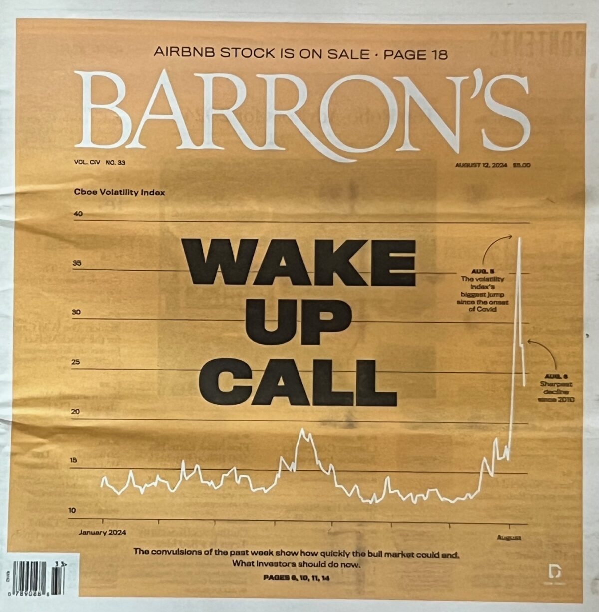
In the past, increases in Implied Volatility have taken much bigger declines in the market for this big of a change. For example, during Covid, the market was down over 30% and the VIX volatility index hit 80 at the bottom after several weeks of large daily declines. The whole world’s economy came to a grinding halt and the market slid with it. At the time it was one of the most terrifying situations the world had seen.
In contrast, at the market’s lowest point on the morning of Monday, August 5, the S&P 500 futures were trading about 10% below the peak they hit in mid-July, and VIX sky-rocketed to 65. It was at less than 30 the Friday before. This rapid expansion in Implied Volatility over such a small timeframe and relatively small index price drop was unprecedented. Option prices multiplied in value and SPAN margin requirements for futures options increased exponentially. Brokers reached out in the middle of the night asking customers to add capital to their accounts, but from where, and how? Since the markets were closed, only minimal amounts of trading was going on and markets froze up with orders becoming unfillable. Trapped traders couldn’t get out, assuming they were even awake and aware of what was going on.
Likewise, the decrease in the VIX volatility index over the next few weeks was also remarkable. By August 16, the VIX index was below 15. Historically, large increases in volatility take months or even years to return to low levels, so this spike from levels of around 12 in early July to over 60 a month later, then back to 15 in less than two weeks is different than anything ever seen before.
For those not familiar, the VIX index is calculated by the CBOE to measure the volatility implied by options on the SPX index with expirations around 30 days away. The VIX index is not tradeable directly, but there are tradeable options, as well as futures that can be bought and sold. VIX is often considered the market’s “fear gauge,” but technically it is an evaluation of how richly options are priced. Since options are priced based on known values, with the only unknown value being volatility, this measure of “implied” volatility impacts all option prices. The numerical value of Implied Volatility of any option is a measure of how much the market expects the underlying security or index to move over the next year, but pro-rated down to the amount for the time left until option expiration.
Margin impacts
Margin works in a lot of ways with options. See the article on margin to learn more. But margin as true leverage is most apparent when selling naked options. For naked short options on stock, ETFs, or Indexes, most margin requirements are based roughly on having 20% of the notional value of the underlying in the account to cover a big move. So, one option contract on a stock trading at $100 would have a notional value of $10,000 and a seller of a naked option would be required to have $2000 for every contract, or would use $2000 of buying power or capital for each contract. If the stock moved 5%, the margin would likely require another 5% of the notional value, which could be as much or more than the premium collected.
If a trader is selling naked options on futures, a different margin calculation comes into play, SPAN margin. SPAN margin is a complex formula, but basically looks at the futures options positions and calculates a worst-case one day move, based on the IV of each option and other factors. This is typically a much lower requirement than what is required for options on stocks and ETFs, so a trader can have a lot more leverage. However, this works both ways. When the market moves, additional margin can be required based on the amount of the move, plus the amount that the “worst case” increased to. On August 5, when VIX spiked to over 60, the worst case scenarios as calculated by the SPAN margin calculation exploded by huge amounts, in addition to losses in holdings that were highly leveraged. As VIX virtually tripled, buying power requirements for futures options also went up by triple or more, when accounting for losses on top of the increased SPAN margin requirements.
Many traders in turn faced margin calls from brokers, asking them to get buying power from negative values to positive. For some the only way to do this was to buy back badly losing positions at big losses at terrible prices with terrible spreads. As much as anything, margin requirements drove liquidation as much as price movement.
The lesson on margin with options from this event is to always have cash or cash equivalent positions that can be easily liquidated to have cash to cover all margin requirements. Even a trader with the worst naked option exposure positions would be alright if their account was 80-90% cash. For me, I had accounts that I had to sell short term bond ETFs to cover buying power requirements on August 5. Every account but one was fine.
Within a few hours of the worst of August 5, VIX dropped significantly, and SPAN margin requirements reduced as well. The question was a matter of whether each trader had enough capital to weather the storm.
Marked loss impacts
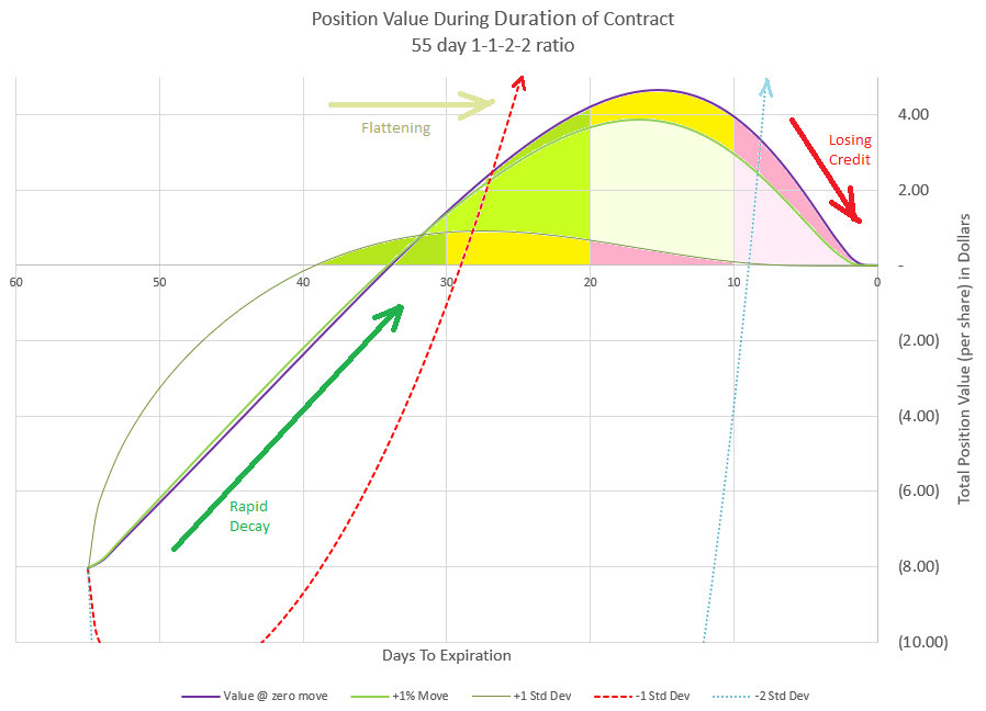
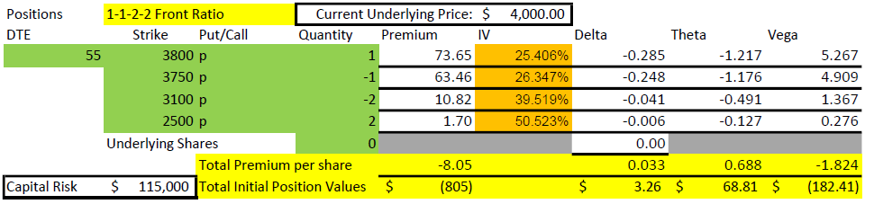
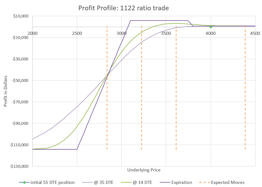
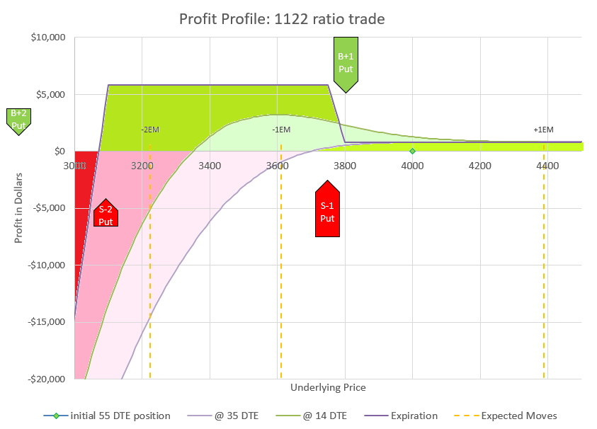
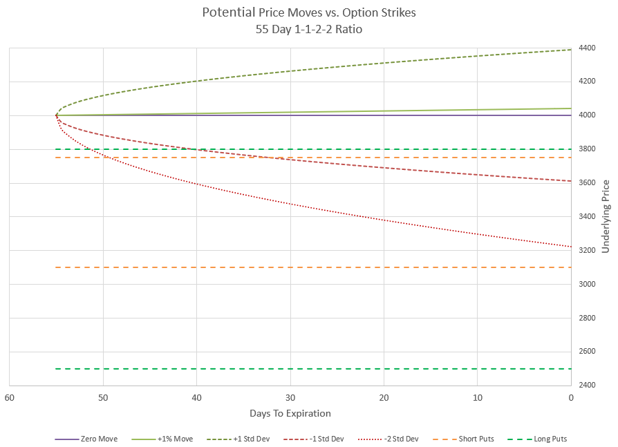
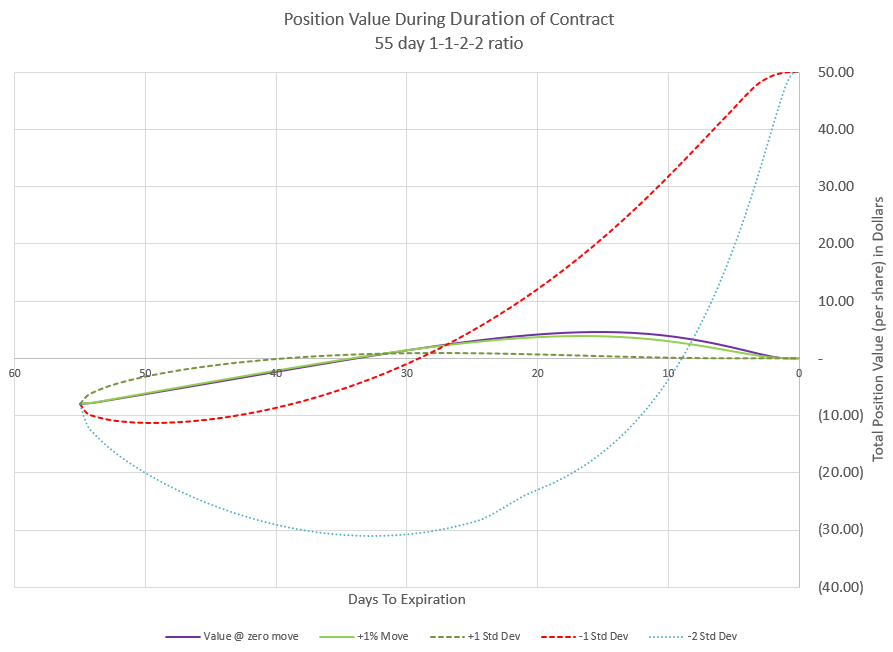
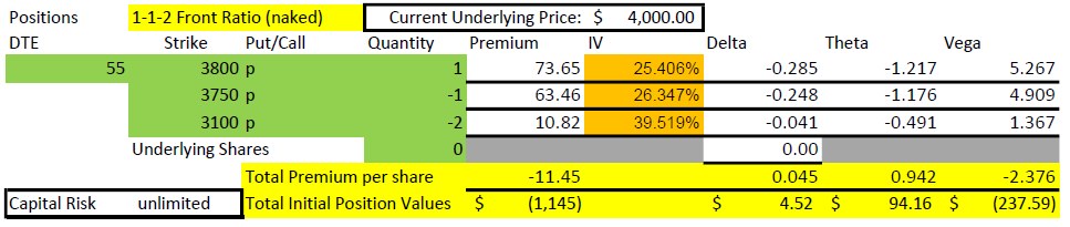
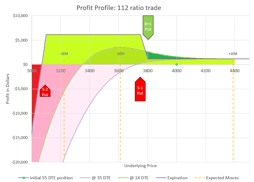
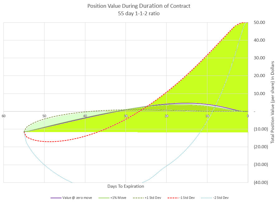
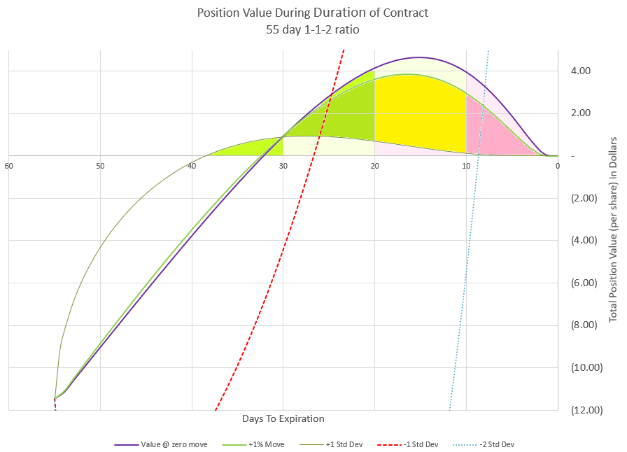
When implied volatility spikes, Vega raises the price of options. On a percentage basis, the impact is greater for strikes further out of the money. For the 112 trade, the “1-1” portion of the trade that includes a 50 point wide debit spread has both strikes increase in price, fairly close to the same amount, while the two far out of the money strikes also rise substantially, but with nothing to cancel out their rise. The overall impact is that the total premium can grow much more than even the percentage increase in Implied Volatility. This is especially true if the positions were opened during a period of very low IV.
So, for a trader that opened a 112 trade when IV was down around 12-13 VIX, the explosion to a VIX of over 60 made the position’s premium value explode to 10-20 times what was collected, something that most traders would never have expected.
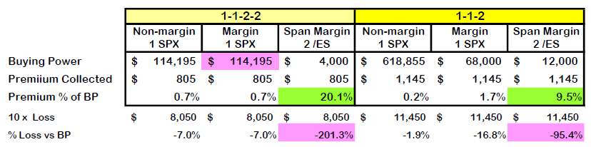
Position size considerations and notional value
With the 112 trade on /ES futures, a trader can use as little as $5000 buying power to control $500,000 of notional value. Even at very low Delta values for the 2 short strikes, it doesn’t take a very big move down to lose way more than the initial buying power. As we’ve just discussed, a big move causes two immediate problems for the trader, a marked loss as premium explodes, and an explosion of buying power requirements.
What is the solution? Keep trades like these a small portion of an account. The vast majority of the time, these trades just decay, leaving the seller with great profits, but when that rare occasion occurs, there needs to be plenty of capital in an account to cover losses and have the ability to manage the position.
Impact of the number of net naked options
I’ve tended to trade mostly covered positions and spreads, where this kind of scenario can’t happen because risk is defined, and a position can’t lose more than the buying power it requires. But it is easy to be persuaded by the siren call of those that tell traders to put on their big boy pants and sell naked options. Somehow, this is considered by some to be the mark of a mature option trader.
Often, traders are told that the buying power required is a good indicator of the risk of a trade. I’ve seen dozens of studies that make this claim. But typically, if you look at the fine print, these studies will say something like naked trades don’t lose more than their buying power 99.5% of the time, or some other high percentage. The problem is that the percentage is not 100%, and that little percent will surface on rare occasions, usually when least expected, immediately after a period of very calm markets.
The key isn’t to completely avoid naked trades, it is to manage the number of naked contracts being traded. During the August 5 event, 112 traders were much more impacted than 111 traders. The difference was two naked puts instead of one. Does that mean traders can load up on 111 and be fine? No, it just means that comparing two trades that both use naked options needs to account for the number of contracts that are naked and the difference in notional value and tail risk. Maybe the 112 trade has a slightly better return on capital typically than the 111. Is the additional risk worth it?
And it isn’t just the naked portion of multi-leg trades that need to be considered. Individual naked trades, as well as strangles or straddles sold naked can be even more susceptible to tail risk. There is a line of reasoning that diversifying will greatly reduce these risks, but in periods of uncertainty and big moves, prices fall across the board and implied volatility spikes everywhere.
Keeping the number of naked positions under control in an account may be the way to prevent a blow-up the next time the market melts down.
Defined risk vs. Naked Risk
If we compare risk of different types of option trading strategies, we can see that there is no risk-free way to trade options, and each risk level has a different set of risk parameters. Probably the closest comparison to selling naked options is to sell credit spreads.
Often, traders confuse the defined risk of credit spreads with being low-risk. In a credit spread, there is the very real risk of losing 100% of the buying power that was required or “defined” by the trade. However, during the August 5 event, the move didn’t impact most traders with out of the money put spreads, because both the long and short strikes of the trade went up significantly in value and if still out of the money, the net premium only went up a portion of the buying power as the moves mostly cancelled each other. Only when prices take an entire spread into the money are worst case scenarios in play. During the Covid crash where the market went down over 30%, this was the case for most spread traders. But on August 5, probably not.
Naked trades on the other hand have no hedge of a long option to provide any protection when the going gets tough. Naked traders are susceptible to both premium increase and buying power requirement increases at the same time when implied volatility spikes, even if the underlying price doesn’t move that far. This is the lesson for naked traders from August 5.
When the tide goes out, you find out who is swimming naked.
Warren Buffet has many famous quotes, and this is one of them. On August 5, 2024, if you were swimming naked with futures options in particular, or even naked options on margin in general, you were probably exposed. I’m not sure that this is exactly what Mr. Buffet meant by this saying, but in this case, a literal interpretation is very fitting.
One time event, or regular occurrence?
What happened on August 5, 2024 was a very unique set of circumstances that came together to create an unprecedented spike of implied volatility. Never before has VIX shot above 60 so quickly, and never before has VIX receded so quickly. So, is this rare event a once-in-a-lifetime occurrence, or will we see similar events on a regular basis?
I’m afraid that we are going to see this type of event many more times. We’ve seen global financial squeezes happen in the past, and this wasn’t even that crazy of a situation. The final straw that broke the proverbial camel’s back with this event was a liquidity crisis in Japan over a weekend. We’ve had other big banking fiascos around the world before and this one may not even be in the top 10 ugliest. What is different is the sheer amount of option positions that are in place now compared to only a few years ago. Today, it is normal for option volume to exceed the number of actual shares traded on major exchanges.
Why does the amount of option volume matter? While shareholders of stocks can simply hold through most downturns, option traders are often leveraged in fairly short duration positions that carry significant risk. When markets change, more traders need to purchase protection or need to get out of losing trades to stop their losses. If this happens when markets are closed, there isn’t much liquidity, and few sellers, so option prices go up, driving up implied volatility. With lots of people wanting to buy to get out or buy to protect, the lack of sellers can cause a panic. This is what we saw on the morning of August 5. Nothing has fundamentally changed since then, and option traders are continuing to grow in numbers.
My fear is that it will take less and less significant events to drive implied volatility and option prices to extreme levels going forward. So, if you weren’t impacted by VIX spike of August 5, consider this a warning shot across the bow. For some of us, they sunk our battleship. Don’t let it happen again.