The first half of 2024 was very good for the 112 strategy. Here’s an analysis of real trades, plus some choices if the market had crashed.
So far…
Occasionally, it’s good to look back and see how a strategy is performing. A lot of traders reach out with questions about the 112 strategy, so it seems like a good time to share some good news. When things are going well, it can be good to review details and see what insights can be gained. It’s also a time to consider what could go wrong in the future. For six months this trade has made money every single time I’ve traded it. That doesn’t happen often with any strategy, so it’s worth taking time to discuss.
I’ve been trading the 112 strategy for quite awhile. I’ve written about it here. That page goes through all the mechanics of the trade, so I won’t repeat that in this post. Instead, we’ll dig into some real world examples and talk about how I chose to manage the trade in a few different scenarios, and answer some questions that I’ve been asked in other forums about worst case scenarios.
A Brief Review of the 112 Strategy
While I won’t repeat the page on the 112 strategy, let’s do a brief overview of what this option strategy involves. Typically, I trade this using /ES futures options on the S&P 500, but I know lots of traders who trade it with other underlyings. I open the trade between 55 and 120 days before option expiration. The three digits of 1, 1, and 2 represent three different put option positions being traded in a ratio of 1:1:2. The 1-1 parts of the trade are buying a 50 point wide put debit spread that costs about $10 to open, and then selling 2 puts that are selling for about $10 each. The net result is that the opening of the trade is around $10 credit. How do I find the right strikes? Just do a little trial and error in the option table to find strikes 50 points apart that are $10 difference in premium. You’ll notice in my results that I actually try to collect slightly more than a net of $10, by picking a put debit spread that is slightly under $10 and selling puts with a premium of slightly more than $10. I usually end up somewhere between $11 and $13 net credit to start. Since I am trading /ES, there is a 50x multiplier, so the actual dollar credit to the account is $550 to $650 with that level of premium.
Most of the time, this is a slow boring trade that slowly decays. If the market goes up, I can usually close the trade for about 20% of what I paid and keep 70-80% of the premium I collected. Often, I only buy back the 2 far out of the money puts, and keep the 1:1 put debit spread in place as cheap insurance. I almost always close the 2 far out short puts early before expiration, usually between half and 2/3 of the way to expiration from when I entered.
Occasionally, the market drops and as long as the drop is not super quick, I can often close the trade for a credit. This happens when the 1:1 put debit spread goes into the money, but the 2 short far out puts have not increased that much. This can get a little nerve-wracking, but this is where big money comes in and why it makes sense to trade the 112 vs just selling one put for $10 out of the money.
On rare occasions, which hasn’t happened this year so far, the market will drop quickly, and 112 positions that are new and haven’t had time to decay will lose money. The 2 short puts will jump in value faster and more than the 1:1 put debit spread increases. If the 2 short puts were ever to get in the money, the losses really explode to catastrophic levels. A trader never wants that to happen. This is what people constantly ask about, and rightfully so- what can I do to prevent my account from blowing up in this situation?
The Results
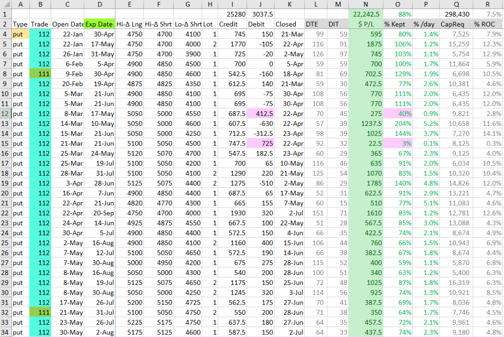
Here’s a table of trades opened in 2024 that were closed by early July. It seemed like a good time to show this concept. There’s nothing special about the sheet- I just made columns for things I thought were important so I could look back later and see what I could learn. Others may track in different ways.
Most of the trades I chose were the 112 strategy, but you can see I sprinkled in a few 111s. The 111 trades were typically entered when the market was a little down and IV was up, giving me a little cushion on entry. You can also see that I varied the DTE entry, with many trades in the 50-65 DTE range to open, and others well over 100 DTE. Longer duration trades use less SPAN margin on futures and allow the far out puts with much lower strikes, but also a bit slower decay.
You can see that most trades were closed between 50 and 75% of the initial duration. In most cases, well over half the premium was kept. I’ve shown the initial premium collected and then the debit that was paid to close, or in several cases, there are negative numbers that mean I actually collected a credit to close, double-dipping with a credit to open and a credit to close.
From the data, you can see three different types of outcomes as mentioned earlier. When the market was on a sustained up move from opening, the trades were usually closed with about 70-80% of the initial credit kept. The trades could have been held to expiration, but closing them or just closing the far out put freed up capital to start new trades. Often, the put debit spread, the 1-1 of the 112 strategy was kept as insurance as there was usually very little value left in those two strikes.
When the market dipped in April, the opportunity came to close several 112 strategy positions for a credit. As price dropped to approach or even go below the upper strikes of the put debit spread, and the far out puts that had decayed already stayed at a low value, the net result was put debit spreads that were worth more than the 2 far out of the money puts combined. I generally watched the Delta values along with Theta to decide when to exit. I didn’t want to let the market get too close to my 2 far-out puts, and I also didn’t want the market to go up past my put debit spread before I closed the trade. You can see several trades that closed in that time frame with a credit, some close to the credit that was collected to start. One trade actually had a bigger credit to close than was received to open. I didn’t try to hold any of these trades to expiration and pin a maximum credit of $2500 per contract- the value of a $50 spread with the multiplier of 50 from /ES, it just never seemed like a position was going to settle there. In hindsight, I don’t think any of them would have- the market came back up not long after I closed the winning credit 112 positions.
There were two trades that are highlighted that were closed for less than 50% of the credit received. These were trades where the market dropped almost right away after the trade was entered. In these cases, when the put debit spread was breached, the 2 far-out puts were also gaining considerable premium. I decided to get out while the trade had a profit and not chance a further decline that could quickly explode to the downside. On one of these positions, I closed the put debit spread, and rolled out the 2 far-out puts to 151 days at a much lower strike, collecting $20 premium and buying a $10 put debit spread for an unconventional trade that closed three months later for a nice profit. So even the “bad” 112 strategy trades turned out okay.
What if…?
Clearly, it could have been worse, and the market could have fallen much faster, leading to big losses. I’m often asked, how can someone manage those kinds of really bad situations with this trade. I have three ways that are very different and each appeal to a different type of trading style.
Set a stop loss, either mentally or with your broker. Many traders I know will set a stop loss at 1x the maximum gain, which for 1 /ES contract of the 112 strategy is typically around $3000. Given that the average gain per contract was around $400, a trader needs at least 7-8 wins for every stop loss just to break even. But considering that it is possible to go a year or more without a loss, that isn’t bad odds. Just know that when the losses come, they are likely to come in numbers, so seller beware.
Define the risk by buying a protective put way below at the opening. This is the whole point of the 1122 and 1111 trades. Losses could be much larger than the stop loss tactic above, but losses are limited to the width between the double credit spread created way out of the money. Some traders add an additional put to make the strategy 1-1-2-3, with the idea that a very, very bad market drop could make the three cheap puts end up worth more than the two short puts- a reality if the market drops 30% within a few months. Besides still having a big maximum loss, adding long puts reduces Theta, so overall decay is slower. But for the once a decade event that crashes the market, this could save a disaster.
Get creative and roll the short put that is being tested way out and down for a credit. Bet that the market will turn around and give back all the losses that were taken. If possible, buy a new 50 wide put spread above the new strikes for $10, creating a new 112 strategy. This is the tactic I used on April 22. It worked out, but I wouldn’t recommend it. Most traders take their losses and move on, and consider this type of loss rolling irresponsible.
So there you have it. A variety of 112 strategy trades from the first half of 2024. Plus a reminder of things that might be done when the market has its eventual down move that is much worse than the little spring dip of this year. Happy trading everyone!
Follow-up note: As with many things, timing is important in trading. Within a few weeks of publishing this post, the market had the fastest spike in Implied Volatility ever recorded, and anyone with significant holdings in naked options, and especially the 112, likely took significant, if not catastrophic losses. In August 5, 2024 pre-market trading, VIX spiked to 65, although the market was only down a moderate amount. Stock traders shrugged, but option traders, especially short in futures options saw premiums explode to extreme levels. Short traders saw margin requirements explode and marked positions move to 10, 20, 0r even 30 times the initial amount collected in losses they couldn’t escape in illiquid markets.
Many seasoned traders I know saw their accounts reduced by 30-50% overnight with their brokers liquidating positions to satisfy margin requirements. In short, the debit side of this trade didn’t provide the promised protection during this event. Many traders, including me, saw big losses even though the debit spread didn’t even go in the money and the short puts were still well out of the money. It was the implied volatility that did the positions in, not the actual underlying market indexes.
I’ve written a separate longer analysis of this situation and the take-aways that all option traders should take from this. While this event was unprecedented, due to the amount of trading now done in options, I suspect that there will be similar, if not worse, events on occasion in the future.
1-1-2 put ratio option spreads are a very high probability trade. The 1-1-2 can be very profitable for sophisticated traders using margin. This trade has very high tail risk for extreme market moves.
I’m a big fan of front ratio type trades. I’ve written about my success with Broken Wing Butterflies and Broken Wing Put Condors. Taking this to a new level is the 1-1-2 Put Ratio trade. This is a new level of ratio trade, because it features naked options with a buffer of protection from a debit spread. The idea is a bit complex to grasp at first, and this is a trade only for traders that have a deep tolerance for risk. The trade involves buying one put and selling a total of 3 puts further out of the money to collect a net credit. Theta makes the value decay quickly, and over time, the purchased put can protect the short puts from most market moves.
I’ve written a separate post on the defined risk version of the 1-1-2 trade, the 1-1-2-2 Put Ratio, while the Broken Wing Put Condor, or 1-1-1-1 is a defined risk version of the 1-1-1, another ratio trade that is very similar. I don’t know of a named reference to a bird or insect for this trade, so I’m sticking with 1-1-2, although I’ve heard some liken the profit curve to that of a whale with a big profit hump and long tail.
I picked up the concept of this trade from one of my favorite traders, “Sweet Bobby” Gaines, who I have mentioned previously in at least one other page on this site. Bobby is a big proponent of the 1-1-2 trade, and has posted numerous videos on it on his YouTube channel, including his recent rising star appearance on Tasty Live. But really, these trades are the next level of evolution moving from broken wing butterfly to broken wing condor to “one louder” as they say in the mythical group Spinal Tap.
What all these trades have in common is selling an out of the money debit put spread, and financing by selling further out of the money puts. The combination delivers a net credit, but also sets up an interesting dynamic of extra rapid decay of the premium involved. The farther out puts decay faster than the closer debit spread, and often lead to the debit spread having more value than the farther out of the money put. This trade takes in a credit to open, and can possibly take in a credit to close. At least that’s how I set them up and manage them.
All these trades are a variation of a front ratio spread, where more options are sold than bought with hedges added to define risk. I’ve also written about back ratio spreads where more options are bought than sold. Front ratios are designed for maximizing decay, while back ratios set up multiple long positions paid for by a costly short position. So what is a 1-1-2?
1-1-2 Basic trade setup
The 1-1-2 takes this a step farther than the broken wing butterly or condor, because we use two puts very far out of the money to pay for the debit spread. The 1-1 part is buying a put around 25 delta and selling a put around 20 delta. The -2 part is selling two puts at around 5 delta. The goal is for the 2 puts to sell for about twice what the 1-1 debit spread cost. I like to set these up with 50-55 days remaining to expiration, quite a bit longer than the other ratio trades I’ve discussed. The added time allows the naked puts to be extremely far out of the money, while still having some meaningful value. I know other traders that go out even farther to over 100 days to get the strike price of the two very far out puts 25-40% below the current underlying price. Like all trades, it’s a matter of personal preference once you know the trade-offs.
What is the advantage of this setup? Well, because each of the two short strikes are further out, we greatly improve the odds of being profitable, and increase the initial rate of decay of the total position. We end up with a big gap between the debit spread strikes and the two short put strikes. Lots of good things happen with this setup. The biggest upside is that there is no upside risk- if price goes up, the trade makes money. The downside of this trade is that it can consume a lot of capital and has significant tail risk, which we will get into before we are done. Let’s look at a typical example.
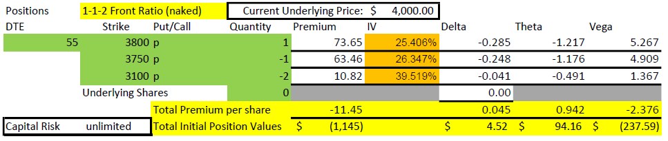
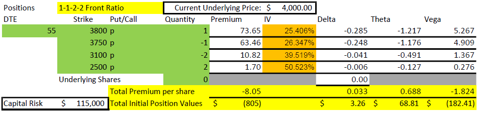
The 1-1-2 trade has two naked puts sold short, but way out of the money.
While this table shows the risk as unlimited, it is actually $618,855, the value of two 3100 puts if SPX went to zero by expiration ($620,000) less the $1,145 collected to start the trade.
Some accounts and some brokers require all trades to be defined in their risk. For example, retirement accounts generally aren’t allowed to use option margin and so any naked put would have to be cash secured. That’s why I’ve written the note about the 1-1-2-2 trade which defines risk to just over $100,000 with two even further out of the money long calls (which is still a huge amount). For this 1-1-2 trade, eliminating those two long puts would mean the max loss would go up to $618,855, assuming that SPX went to zero, while we are holding two short 3100 puts. SPX will only go to zero if we see modern society end, and in that case, we’ll probably have bigger problems than our option positions. But rules are rules, and so if you want to trade without the long puts in a retirement account, you would need $620,000 capital to make a likely $800-$1200, or less than 0.2% return in 55 days or less, probably not the best use of capital. We’ll discuss other alternatives after we review the details of the 1-1-2 trade.
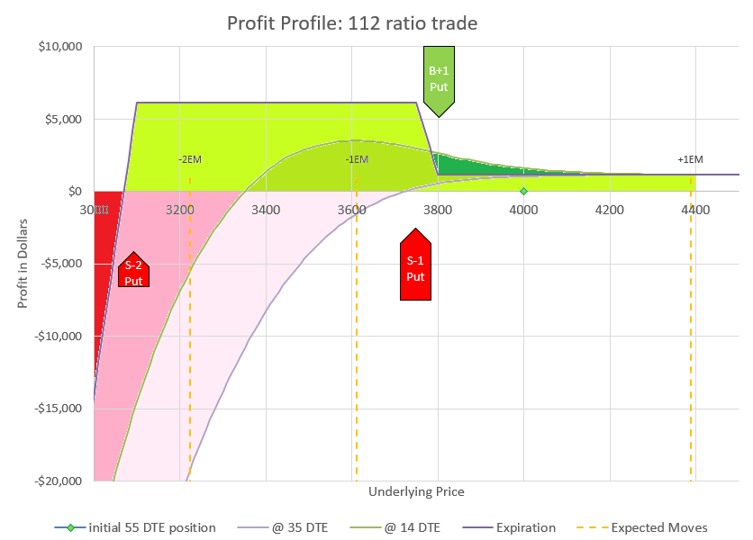
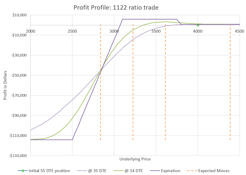
The profit profile for the 1-1-2 is very similar to the 1-1-2-2 other than the virtually unlimited loss.
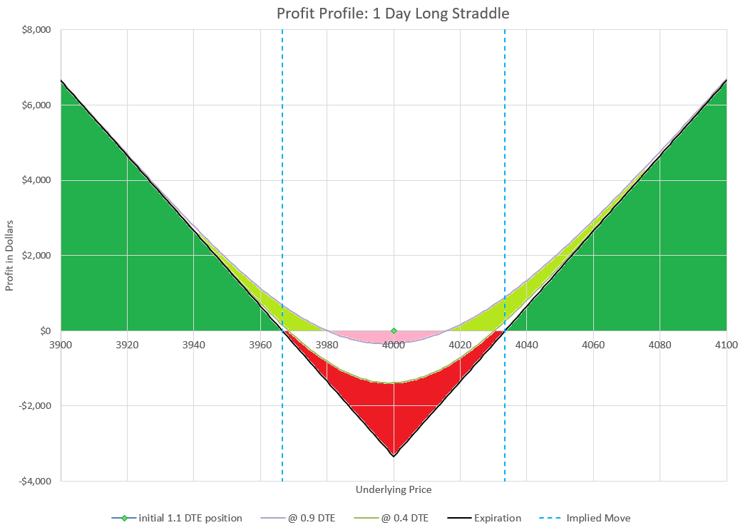
This chart shows how changes in the underlying price will impact the profit and loss of the trade. We evaluate at four points in time. The green diamond shows our initial position at 55 DTE, underlying price is $4000, and the P/L is zero. The curvy lavender line shows how price would likely impact the position with 35 DTE. The green curve shows the likely profit at 14 DTE, and the sharp purple lines are the expiration values. We know exactly what expiration values will be at any price, but the curves are estimates based on likely impact to implied volatility as time passes and prices change.
The first thing I want to point out in this example is that the 3100 short put is 900 points below the current price of $4000. For that strike to get in the money, it would take a 22.5% decline in the market in 55 days. That won’t happen very often. To be fair, this example uses values with VIX at 25, a historically higher than average value, but for the timeframe of 2020-2022, a fairly middle of the road level. The higher that implied volatility is, the farther away the short strikes can be and still collect meaningful premium.
The next thing to point out in the setup numbers is the Greeks. Delta is fairly flat at +4.5. For a credit trade, that isn’t much and means that the position can handle some movement in price. Theta is $94/day, and we collected $1145. So, the position is expected to lose 1/12 of its value each day. But we have 55 days, so how does that work? Quite well, I’d say.
Remember that our starting underlying price is $4000 and the trade is profitable at expiration as long as price is above 3100. The chart above doesn’t show losses all the way down to zero price, but just imagine zero price and -$618,855. Our probability of profit is 96% if held to expiration based on the Delta of 4 for the naked puts.
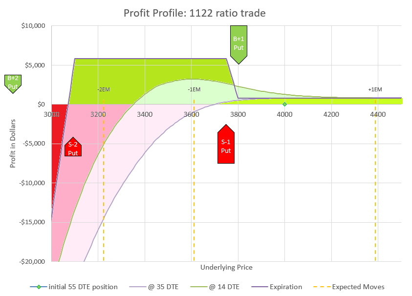
1-1-2 Trade Expected Move Analysis
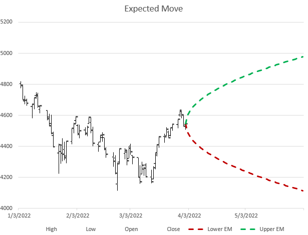
I’ve put in dotted lines to show the expected move and multiple expected moves down. If you need a refresher, check my earlier post on expected moves. It is likely that price will end up inside of one expected move, the dotted lines on either side of the current price of $4000. There is approximately a 2% chance that price will move two expected moves to the second dotted line below the current price, which would still be max profit for this trade at expiration. And there is approximately a 0.3% chance of moving three expected moves to the far left dotted line. We can go further, but the odds keep dropping as we go to lower levels. However, as history has shown, moves down tend to have somewhat higher probability than theoretical probabilities once we get beyond two expected moves. The point is that this trade is very likely to end up profitable, but there is risk that an extremely big move down could lead to an extremely big loss. We’ll talk about ways to reduce exposure later.
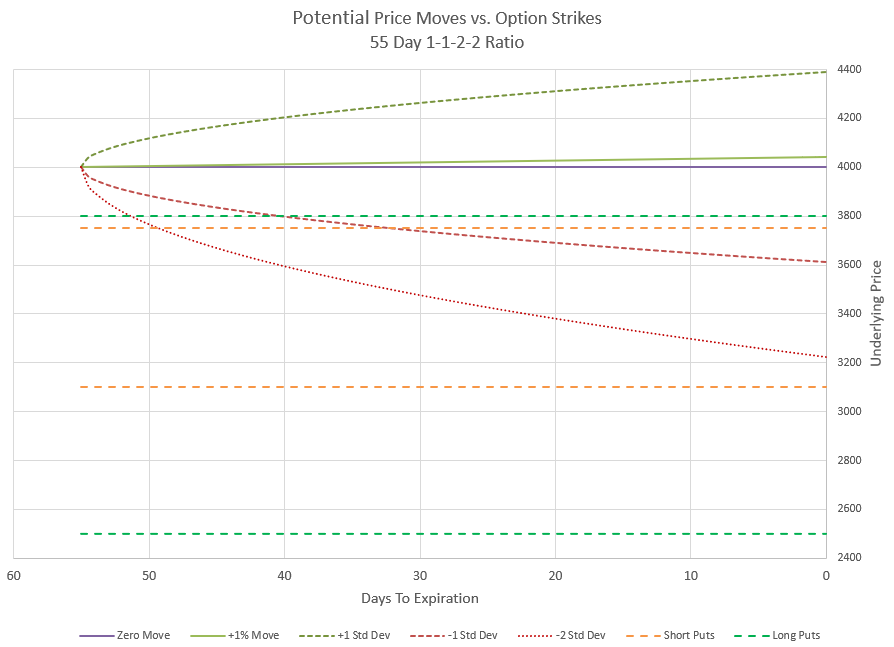
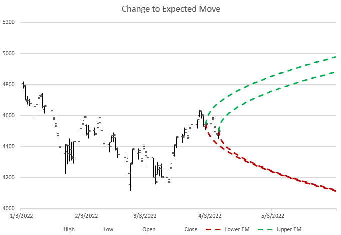
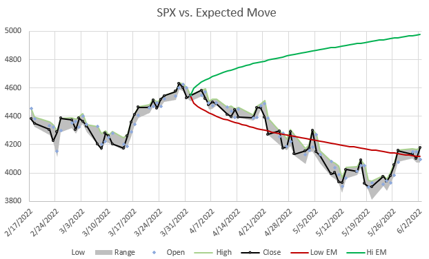
Let’s look at this another way. Prices don’t generally move immediately to a new level, but have probabilities of moves that get bigger over time. Again, going back to expected moves, let’s compare how we might expect price to move during the duration of the trade.
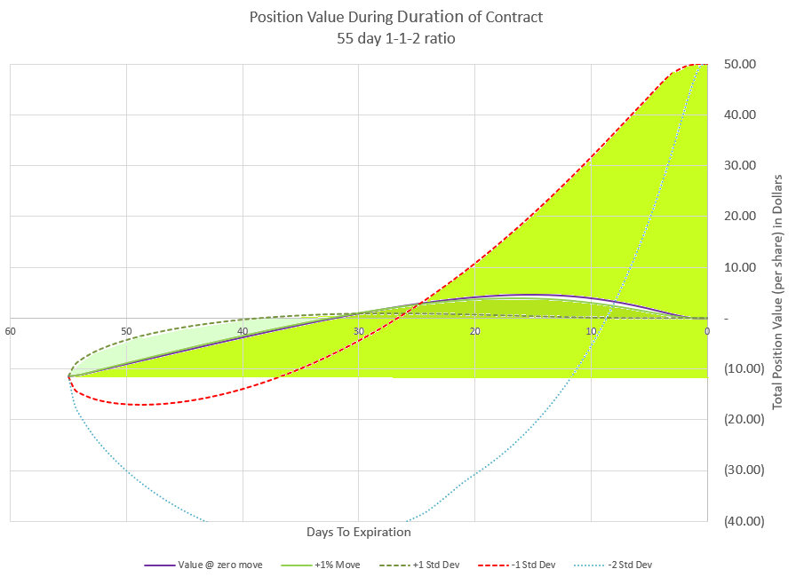
This chart shows expected moves day by day from initiating the trade until expiration, and compares to the put strike prices.
In this chart I’ve shown several outcomes. The zero move is if price doesn’t change at all, a baseline. I’ve shown a +1% move which is in line with the positive drift of the market. There’s also a line for the positive expected move and the negative expected move, where price is likely to be within at any point in time. And finally I’ve shown a curve for a price move of two times the expected move down. Notice where the strikes are relative to the price curves are. The negative curves take time to get below the upper 1-1 put debit spread strikes, and never reach even the short put of the 2 further out short puts. This chart also shows where two even further out long puts would be placed for a 1-1-2-2 version, but that’s covered in the post for that trade. For most people trading this strategy, defining risk with deep out of the money puts doesn’t provide a lot of protection as it is extremely unlikely that those puts would ever be in a position to reduce the level of a loss as this chart clearly shows. So, let’s not dwell on them.
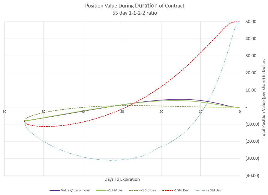
Now let’s look at what happens to the value of our premium if price were to follow each of these curves. This is a view that you don’t see much because it is based on lots of assumptions for the pricing models. Since implied volatility is not predictable in the future, we have to guess how it will change if underlying prices change and how that will in turn impact prices. Based on how price changes have historically impacted implied volatility, we can have a decent estimate of how it will likely change with future price changes. I’ve used a model to take all that into consideration for these position value charts.
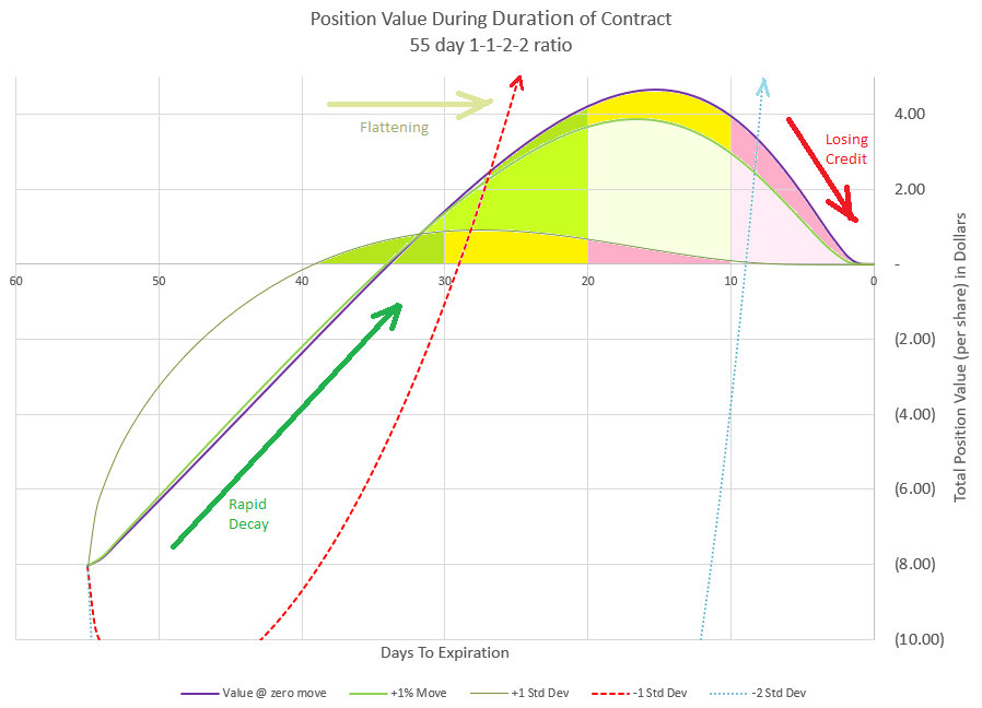
Most scenarios eventually show a profit with 1-1-2. Note that this chart shows position values, not profit. All values start with a value of -11.45 (the opening credit); the green shaded areas represent profit.
Looking at 1-1-2 values over time at the same price moves that we looked at for the expected move multiples, we can see that the premium changes are fairly dramatic and more positive as expiration approaches if the market is down.
Initially, this position collected $11.45 in premium, so we start with a negative or short value of -11.45. From there the price moves shown in the previous chart drive the premium up or down along with time decay. If price is flat or going up, premium decays and moves quickly toward zero premium. If the price goes down, the positive Delta pushes premium to more negative values. The price move of negative two expected moves really does a number on our premium initially, driving it down to below -40.
But, remember our profit chart at expiration? The flat and positive moves end up with a profit of our initial premium (all the puts have zero value at expiration, and the negative expected move and negative double expected move end up at maximum profit. Since our debit spread is 50 points wide, the negative moves would leave it fully in the money for a premium value of +50 points. And that’s in addition to the initial premium collected to open the trade. The challenge is that to get that max profit, we likely will have points in time where our position loses money.
The probability of getting to max profit is low because it would require a price drop between 6 and 22%. Based on our put strike Deltas we can estimate that we have about a 20% chance of that. Most of the other 80% is expiring with all strikes out of the money. So, it might be wise to zoom in and understand what happens with the vast majority of trades.
Zooming in on most likely outcome’s value over time
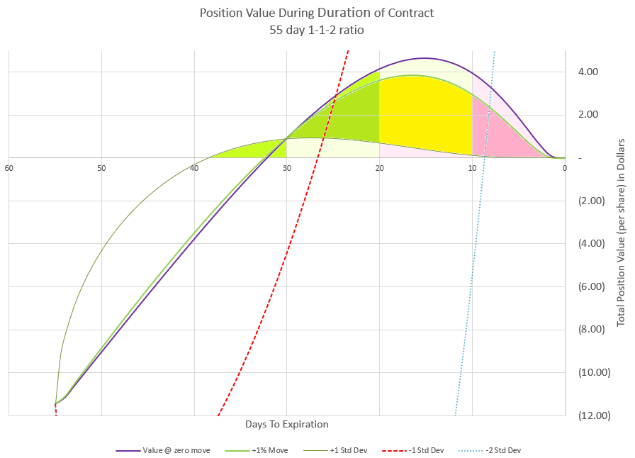
If we zoom in on the likely outcomes with the market being flat to up, we see that premium behaves very uniquely during the life of the trade.
If price goes up or drops less than 200 points, we can keep our initial premium at expiration. We may be able to collect more. The profit curve at 14 DTE is actually above the expiration profit if the price remains the same. How is this possible? Because the 1-1 debit put spread decays slower than the 2 naked low Delta puts, eventually the 1-1 part is worth more than the -2 part, even though the -2 part started out with twice the value of the 1-1.
I used this chart as the featured image of this post because I thought it best illustrates how this trade plays out most of the time. If you remember when we discussed the Greeks, I pointed out that Theta is very high compared to the premium. From this chart we see that if price stays the same or is slightly up, premium will decay to zero by 32 DTE, or just 23 days into the trade. This is an example that Theta isn’t 100% accurate by itself as it looked like 12 days of Theta should move us to zero value. From the chart you can see that the curve is fairly consistent for no underlying price movement as the value of the 1-1-2 position approaches zero, but still we have very rapid decay that I don’t think anyone can complain about.
Like all ratio style trades we have discussed, this trade has the possibility of switching from negative to positive premium. The difference with this trade is that it is actually quite likely, and as such we need to plan for it and manage our profit accordingly.
I’ve colored in the area under our three flat-to-positive curves with three zones each. There is a green zone where positive premium is growing, a yellow zone where premium is topping out, and a red zone where positive premium is being lost. Notice that the curve of the 1% up move and no price move are fairly close together, and that’s because the price movement is relatively close to the same compared to the other moves we are analyzing.
Let’s review how this happens. This trade essentially has two components, a slow decaying debit spread (1-1), and a fast decaying pair of deep out of the money naked puts (-2). The two naked puts decay faster because they are way farther out from the money, and have twice the value to start with than the debit spread. All these factors help decay happen more quickly. As long as the price stays fairly stable, this relationship will hold. Theta will be the primary driver of the premium value, and the low Delta naked puts will get to be worth less than the narrow debit spread.
The most likely scenario is that we stay inside the expected move and travel somewhere close to the no price move or 1% up move. Let’s realize that the market doesn’t move in equal amounts every day like this chart, so think of it as a smoothed out version of what premium would do. In the real world, premium would bounce up and down with price. However, if our price is close to where we started with 20 days until expiration, we would expect that the premium switch to positive has about maxed out, and it is probably a good time to close out the trade. Hopefully,your trading platform has a analysis feature that lets you look at your position and see how profits are changing day by day to help determine when the position is as high as it can go.
Without a chart, another way to determine how close the trade is to switching direction is to watch the position Theta. At the beginning of this trade, Theta was 0.942, or $94.16 for the full contract per day. As the trade progresses, Theta will decrease and at some point when the premium goes positive, Theta will turn from positive to negative. As it gets close to zero, that is the peak premium value. I generally try to exit the trade a few days before Theta is projected to turn negative. A big up day for the market could quickly change my very positive premium to not as positive premium, so it isn’t a time to get greedy.
So that brings us to the curve for the positive expected move. This is the curve that assumes that the price follows the one standard deviation move up. The good news when this happens is that premium decays very quickly because Delta and Theta team up. The not so good news is because the price move gets so far away from the strikes, the total position won’t get to a very high positive value. This is because all the options will drop in value quickly, approaching zero, and the upper debit spread won’t have much value. A big move up means that the probability of any of the strikes going into the money will be very low, so there is very little premium. As a result, it is likely we won’t be able to get out for much positive premium if any at all, but we will be able to keep most, if not all the premium from the opening trade. This is the least stressful outcome of the trade. If the price moves up faster than the expected move, premium will likely drop to very close to zero and may not ever go positive. So, if price is up a lot and the trade can be closed for a credit, I take the money and run. I’m happy to have a quick, winning trade.
As the trade progresses another helpful element is that Delta tends to reduce to zero or even become negative as time goes on if the underlying price stays close to flat. If a trader adds on many of these trades with different expirations, the overall position tends to be fairly low Delta and trades that have been in place for a while can buffer more recent positions. This is true until a really big move down hits and tests the naked puts. Then Delta grows quickly making losses pile up quickly as down moves continue.
The risky negative outcomes of the 1-1-2 trade
Looking at the position vs time value chart, there are two lines that represent what happens if price goes down. One is the move down one expected move and the other is down two expected moves. Interestingly, in this example, both end up at max profit by the end of the trade. So, it would appear that the trade can’t lose, which is far from true. Notice that these premium values may go very negative if prices drop quickly after opening the trade. This is because the narrow debit spread doesn’t pick up as much value from increasing delta as the wide credit spread does in a down move. We know that if price stays above our credit spread short strike at expiration, we will make money, but when price moves quickly down, it isn’t clear that price will level off.
So, as a trader, we are left with a choice when the market drops, We can take a loss and get out of the trade, or wait to see if the market quits dropping before it tests or violates the credit spread strikes. If we are a week or two into the trade, a decent down move will not make a huge impact, but initially the trade can take a big hit from a down move. The longer we are into the trade without a big down move in price, the less the risk is of a loss. On the flip side, a big move down opens the possibility of additional big down moves that can lead to a very big loss. We reviewed the odds earlier- about 4% of the time the trade will lose based on the far short puts having an initial Delta of 4. If this trade is done enough times, there will be some losses. Let’s look at some management actions that could be taken.
1. Set a stop based on premium price. In this example, we collected just over $11 premium to open the trade. So, we could set a stop to avoid losing twice ($22) or maybe even three times ($33) our initial premium. This would mean a stop loss if premium climbs to $33 or $44, given that $11 premium is our starting break-even point. This is the simplest risk mitigation strategy. Using this will lower the overall win rate as many negative scenarios would end up fine if not closed, but this management technique will prevent huge losses that might impact the account dramatically.
2. Close the trade if the underlying price goes below a trigger point. We know this trade has a lot of cushion. We can handle much more than one expected move and be profitable. But if the move is much more than expected, we have to consider that the move is very unusual and dangerous for us. Perhaps our point to get out is when the debit spread is in the money, or when we are half-way between the debit spread and two naked puts. Or maybe it is the strike of the short naked puts that is the final trigger to get out. The further down we allow price to go down, the more we stand to lose. Pick the underlying price where it gets too uncomfortable and use that as the trigger point to get out of the trade.
3. Roll out in time if premium or price triggers are hit. If the position is rolled, it can be rolled out for a credit. This gives more time for the market to turn around. However, it gives more time for a losing trader to lose more, because we likely can’t roll down much lower and still get a credit, and we will likely have to pay to roll the debit spread. If the price move continues down, there will be much less room to maneuver going forward.
4. Simply hold on and hope the probabilities play out. With 55 days in the trade, we just need to move down less that two expected moves by expiration. If the capital is available, and the conviction is there, holding can bring max profit with a big down move. Note that as time passes and the naked puts stay out of the money, the premium has to go away, so the value can evaporate very quickly with very high Theta as expiration approaches. This can be observed in the value vs time graph for the -2 EM curve. It can also result in a very large loss. As expiration approaches, the difference between max profit and a much bigger loss is just a few percentage points of price movement and the potential loss is much more than max profit.
In this example we can see that a move down of one expected move really doesn’t challenge our position, while two times the expected move is playing with fire. So, one approach might be to hold as long as the move stays within the expected move to the downside and switch to closing or rolling once the move exceeds that or some other multiple of expected moves. In any case, a trader has to know their risk tolerance and have a management plan for both winning and losing trades.
What about calls?
A logical question might be- if this works so great for puts, why not double up and do it for calls as well? Well, there’s one problem- skew. On indexes implied volatility is higher as strikes go to lower values and declines for higher strike prices. As a result, out of the money puts have higher implied volatility than out of the money calls. More importantly, far out of the money puts have higher implied volatility than puts closer to the money.
Look at our setup for this example. Implied volatility of the single long put is around 25, while the two short puts have implied volatility of 39. This helps two ways. The short puts have more of their premium tied to volatility, bumping up their price compared to the long put. Also, the higher implied volatility pushes the strike price further down to get a matching premium to the debit spread, making the trade a higher probability of success. We are selling more of the higher implied volatility and buying lower implied volatility, a key reason to use front ratio spreads.
A similar setup for a 1-1-2 call trade would reverse the dynamics. The long call closest to the money would have the highest implied volatility and the two short calls would have the lowest. To collect similar amounts to the put trade, the call strikes would be much closer between the debit spread and credit spread, and the difference in the deltas of the strikes would also be closer together, meaning a narrower window of max profit, and a higher probability of max loss. While still a trade with positive probability, it generally isn’t as attractive as the put side.
Buying power requirements for 1-1-2
I usually don’t spend much time talking about buying power because most trades I do are defined risk credit trades where the amount collected is a significant portion of the capital at risk. This trade is not so much, as it is a naked ratio spread (1-1-2). In non-margin accounts, we collect 0.2%, which isn’t much.
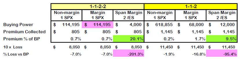
Below is an analysis of different possible ways to trade. I looked at trading each of these strategies three different ways. First, I looked at a cash secured account, like a retirement account. Next, I looked at an account with margin for naked options. Finally, I looked at a much different approach, trading futures options with span margin. The margin and span margin amounts came from entering this trade into the tastytrade trading platform. I’m also showing the defined risk 1-1-2-2 version for comparison as well.
Comparing buying power impact of different account types for the two strategies
I highlighted some key takeaway points. First, is how leveraged span margin with futures options can be for this trade. Our most capital efficient trade would be doing the 1-1-2-2 on futures span margin where we would collect 100 times the premium as a percentage of buying power (20%) than the non-margin account of the 1-1-2 trade (0.2%). Of course, with leverage comes much more risk. I chose to consider a loss of 10 times the initial credit as a practical worst-case scenario. The span margin would end up costing huge amounts more in a disaster and could potentially wipe out an account if the trade used a high percentage of the account’s capital. Span margin isn’t static, when a trade moves against a position, the span margin is re-calculated and the requirements can quickly explode in a big market move.
A couple of weird margin anomalies to point out. In my margin account, the defined risk 1-1-2-2 trade required almost twice the buying power as the undefined 1-1-2, which is weird because clearly there is more risk in the naked 1-1-2. I think it may be that the calculation for defined risk is normally much less than undefined and the software may just assume that margin is not useful in defined risk. On the other hand, defining the risk on the futures version cut the buying power by 1/3. Different brokers may calculate their margin requirements differently, so don’t take this as universal truth. Similarly, remember that while defining risk usually increases the return on capital, it makes outsize losses more likely, especially when scaling up. Notice that the highly leveraged futures 1-1-2-2 would lose twice as much as a percentage of capital that the futures 1-1-2 setup in a 10x loss. I discussed this phenomenon in detail in my post on comparing risk.
Remember that margin and span margin change as the trade progresses depending on the market behavior. Span margin is subject to big swings when prices go against a position. A broker may force a position to close much earlier than a trader would want to get out due to expanding capital requirements. So, while initially the position is cheap to enter, a trader needs to limit each position to a fraction of the overall account size.
But the good side of this is that this trade can be entered for a very small cost. The trade is very high probability. We can also make more than the premium collected. I didn’t include it in the chart, but maximum profit for the most leveraged choice above would be $5,805 profit on $4,000 buying power, a return on capital of 145%. And there is over a 20% probability of that happening.
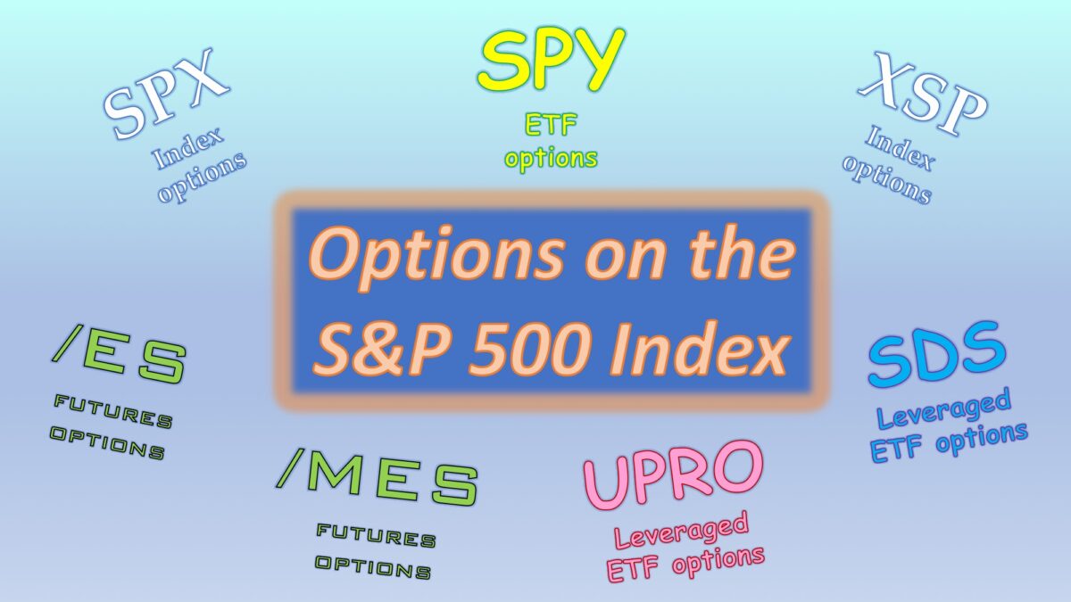
One final note on the buying power analysis table. To keep the quantities an apples-to-apples comparison, I used double the number of /ES futures options because futures options only control half as much value as SPX index options. So, technically, those futures options trades listed are 2-2-4-4 and 2-2-4 because they use twice the number of contracts to get the same notional exposure. I reviewed differences between index options and futures options in detail in my post about different ways to trade options on the S&P 500 index.
What about small accounts?
Readers looking at this may be thinking, “Gee, this is great for multi-millionaires, but what if the account is too small to consider any of these buying powers?” Great question- there are other alternatives. First off, a trader could use half the buying power listed by just trading options on one contract of the Mini S&P 500 futures (/ES). The 1-1-2 example would only take $6,000 buying power for $572 premium received. But, if that is still too much, we can make it a lot less.
Many traders are more familiar with options on the SPY exchange traded fund, which trades at approximately 1/10 the value of the S&P 500 index. For futures options, there is also options on the Micro S&P 500 futures contract (/MES), equal to 1/10 of the /ES contract size, or 1/20 of the size of an SPX option. By using SPY or /MES, we cut the size of the trade down by 1/10 compared to the above table. If the account is taxable, another choice would be the $XSP index, a 1/10 value index of the S&P 500 with favorable tax treatment, but much lower liquidity with few options that far out in time. Again, all these alternative versions of S&P 500 options are discussed in my post on different S&P 500 choices.
So, for an account with futures trading capability, this trade could use /MES futures options and get into the 1-1-2 trade for just $600 buying power. An account with options margin could use SPY or $XSP and get into the 1-1-2 trade for $6,800 buying power. A trader doesn’t need a million dollar amount to trade this.
Concluding thoughts on 1-1-2 trades
I know a number of people who have traded versions of this trade during the bear market of 2022 without any issues. One trader I follow and interact with had one of their best years in 2022 because of this trade and the bear market that moved the market down, but not fast enough to ever drive the naked puts into the money. In fact, it could be argued that this trade, like most trades that collect credits from selling puts, works best if entering when the market is already down and implied volatility is high. Bad scenarios are already priced into option premium and there is a lot of cushion between strikes. This trade is most dangerous when volatility is low and prices are high- the probabilities are not as good, because a move of more than two times the expected move down is not nearly as far.
While not for everyone, the 1-1-2 trade provide a very high probability of success with a nice payout when used with leverage. The trade requires monitoring to maximize profit and to prevent catastrophic loss, so it really is not a set it and forget it trade. The key is to have a plan to manage the position if the market goes against the trade and stick to the plan.
Many people are buying and selling options with zero days to expiration (0 DTE in option lingo). But is this a good idea? Are there strategies that actually work? Or is this just gambling? Well, like many things in options, it depends. There are strategies that have been successful with years of history, and we’ll dig in to discuss them.
In 2022, the option exchanges rolled out options on a few indexes that expire every day of the trading week. This has caused a frenzy of option trading by individuals who are trading a variety of expiration day strategies every day. Many people are buying and selling options with zero days to expiration (0 DTE in option lingo). But is this a good idea? Are there strategies that actually work? Or is this just gambling? Well, like many things in options, it depends. There are strategies that have been successful with years of history, and we’ll dig in to discuss them.
Over the past several years, the frequency of option expirations has increased dramatically, particularly for the major indexes, the S&P 500, the Nasdaq 100, and the Russell 2000. Initially, there were only monthly expirations that expired on the third Friday of the month. Options expiring every Friday were added several years ago, and Monday and Wednesday were added a few years back, and finally in 2022, Tuesday and Thursday expirations were added. Trading volume has grown exponentially, and trading on options expiring within the next few days are now the majority of option trades. Clearly, expiration day trading is very popular.
I’ve been exploring trading strategies for expiration day for several years, going back to when we started having expirations available for Monday, Wednesday, and Friday. I’ve discovered that 0 DTE is not for everyone, can have many elements of gambling for many, but has a few strategies that have a positive expectancy of profit.
Things to know about 0 DTE
First off, 0 DTE requires a different mindset than longer duration trading. Profits and losses explode in minutes, making the importance of having a plan critical. Options in general require strategies and planning, but 0 DTE is significantly more volatile. So, for traders that can’t handle huge swings in value over very short periods, 0 DTE may not be a good place to go.
For traders that do trade 0 DTE, I highly recommend keeping a log of all trades to be able to evaluate whether the strategy being used is actually working. Some trades have fairly high win rates, but have big losses when they lose- a log will help a trader determine if the wins outweigh the losses over the long run. Also, keeping note of what went well and what went wrong will help a trader learn from success and failure. I can tell you that most traders that fail do so by not sticking to their own rules for managing risk.
One key consideration is the Pattern Day Trade Rule that applies to accounts with less than $25,000. Federal regulations prevent small accounts from opening and closing the same position the same day more than three times in any 7 day period. Doing so will place severe limits on the traders account. If you have an account with $25,000 or less, or even just slightly more, you need to be very aware of this rule and how it works before even thinking about 0 DTE trading or any short duration in and out trading strategies.
There are a number of ways to trade 0 DTE. Some traders try to get in and out, while others hold a trade to expiration at the close of the day. Some are net buyers of options, what I will call debit trades, while other are net sellers, or credit traders. I say “net” because many strategies involve trading spreads, buying one option and selling another, generally the more expensive being hedged, protected, or partially financed by the cheaper option.
When options are expiring at the end of the trading day, all the characteristics of options are sped up. From a data driven standpoint, there are three key Greeks to consider. The two most obvious are Theta and Gamma which essentially battle it out for the day. But Vega also plays a key role, as big moves spike up Implied Volatility and option’s premium, and calmness can sap premium almost as fast. With hours or even minutes until the options expire, the Greeks’ calculations stop meaning as much as the concepts behind them.
Options sellers are banking on Theta eating away the premium as the day progresses. If the option ends out of the money at the end of the day, it is worthless. On the other hand, Delta will end the day at either 100 or zero and is likely to swing huge amounts during the day, which is the measure of Gamma, the change of Delta. So option buyers are looking for options to get in the money and run way up in value.
Since we are talking about expiration, it is important to understand the implications, which vary depending on what underlying the option is based on. Remember, there are four types of underlying securities, and at expiration the differences really stand out when an option expires in the money. For stock and ETF options, in the money options are settled with shares, which may not be the best outcome for day trading. In addition, while expiration option trading ends at the closing bell, expired stock and ETF options can be exercised until midnight, so even options that end trading out of the money still might be exercised if market conditions change after hours from news or earnings impact. Index options are much more straightforward. Index options are cash settled based on the price of the index at the closing bell. Because of this, index options, like SPX, are generally the preferred trading vehicle for traders holding options through the closing bell. Futures options settle with futures contracts unless the futures contract is also expiring the same day. However, futures options are assigned based on the price at the closing bell, not any after hours moves, so a trader knows at the bell whether there will be an assignment or not. So switching between underlying types for 0 DTE trades in not a trivial decision.
As mentioned before, because 0 DTE trades can rapidly change in value, having a mechanical trading plan becomes critical for consistent success. Most traders that trade short/selling strategies use stop losses to keep losses from getting out of hand, and long/buying strategies use some type of trailing stops or rolls to protect winning positions and keep upside unlimited. There are a few trades where holding to expiration (no matter what happens) could be considered, but I think 0 DTE are best managed by active trading based on market action.
So let’s get to it. Let’s discuss some typical strategies, both from the long and short side, considering what it takes to be successful.
Selling options with 0 DTE
Most 0 DTE option sellers I know actually sell spreads to define risk. Selling naked options on expiration day simply requires too much capital and carries too much risk for the average trader. The width of the spread can vary based on the strategy or capital available to the trader, but wider spreads tend to decay faster than narrower spreads. These trades are expected to win a high probability of the time, but to avoid severe losses, stop losses are also critical parts of the strategy.
While there are many variations of these strategies- different times to enter and exit, trading one side or both sides (puts and/or calls), entering or exiting all at once or legging in based on the market, the core of the strategy is the same. Sellers want to sell at a relatively high premium and buy it back for less or even let it expire worthless. I’m going to focus in on two common strategies that I have had success with and 0 DTE trading friends have done successfully- a wide Iron Condor and an Iron Fly. For discussion, let’s assume that we are selling spreads directly on the S&P 500 Index, ticker symbol SPX.
0 DTE Iron Condor
Iron Condors on expiration day seem to perform best way out of the money, selling options with 10 Delta or less and buying 30 to 100 points further out of the money. Greek calculations for 0 DTE can be flaky and vary widely, so many traders are more comfortable choosing strikes based on the premium available. For example, a trader may sell the lowest put strike that sells for over $1.00 or maybe over $1.50, and buy the put that sells for under $0.75 or $0.50. For perspective, you can estimate the expected move at any time in the day by adding the premium of the at the money put and at the money call. Generally, these strikes are between 1.5 and 2 times the expected move for the put being sold and another half expected move further for the put being bought as a hedge. So, it’s highly likely that the strikes will expire worthless.
Similarly, we do the same thing on the call side, selling a call and buying a higher strike call for less. If we choose similar Delta values, the premium for each call will be less, but the difference in premium may actually be more if we have the same width wings. It is a matter of preference as to whether to try to collect as much on the call side as the put side.
The risk vs reward for this set-up is the net premium difference between what was sold and what was bought and the difference between strikes. For example, if we sell a put for $1.50 and buy a put at a strike price 40 points lower for $0.70, we are risking 40 to make 0.80. Then, if our calls were sold for $1.20 and bought for $0.40, we have another 0.80 on another 35 wide spread. So in total we have 1.60, but still only 40 risk because the options can’t expire in the money on both sides. Actually, because the options are for a multiplier of 100, we risk $4000 to make $160. So, if all goes well, we make a 4% return on the capital needed in one day. Some traders sell slightly closer strikes to try to collect more premium, and others sell for less to improve probabilities.
While probabilities are fairly high that the strikes will end up out of the money, we never know for sure, so we have to protect our capital. Most traders I know use a 2x stop loss on each side. They limit their loss to twice the premium they collected on each side. So, if a put was sold for $1.50, losses are limited to $3.00 by entering a stop loss on the short put at $4.50. While a stop can be entered for the price of the spread, it isn’t recommended because during the day prices can vary in weird ways and stops can trigger on spreads when the price hasn’t really moved much. I’ve read numerous posts of traders who were frustrated by a stop that was executed when there position was in no danger because of a rogue quote. If possible, it’s best to have the stop trigger based on the bid price of the option if your broker allows it- for the same reason- to avoid bad quotes triggering a stop.
It can be frustrating when a stop triggers just as the underlying price hits the high or low of the day and reverses. A trader looks at this and thinks, “Gee, if I wouldn’t have triggered the stop, my option would have expired worthless. I took a 2x loss when I could have had a gain.” Unfortunately, a trader never knows when the price will reverse and when it will keep going. The goal is to stop our loss at 2x and not let it get to 10x or 20x. We can recover from small losses, losing all the capital of a spread trade can be devastating.
The Iron Condor is a 4 legged trade, so if one leg is stopped out, we still have three legs. On the side where the stop occurred, the long position will have gained value, although not as much as the short strike lost. We can hold the long strike in the event that price keeps moving, making the long strike more valuable. However, since the strike is likely still well out of the money, it is likely to expire worthless and probably is best to be closed out soon after the short strike stop occurs.
When we are stopped out on one side, it is even more likely that the opposite side will expire worthless. However, there is a small possibility that price action could reverse and move far enough to stop out the other side as well. For that reason, some traders will close out one side if the net premium has decayed 80 or 90% of the way while there is still a lot of time left in the day. The choice is take risk off the table, or hold out for that highly probable last 0.25%. Again, it’s personal preference.
So, let’s look at the various potential outcomes of our $1.60 Iron Condor: 1. most likely (~70%) both sides expire worthless $1.60 profit 2. sometimes (~25%) one side is stopped out and the other expires worthless ($3.00 loss on short stop, $0.20 gain on long, $0.80 profit on other side) $2.00 loss 3. rarely (~5%) both sides stopped out, assume no net gains from long strikes so $6.00 loss ($3.00 each side) Adding all the probabilities together, we get an average return of 0.33 profit, or $33 on our $4000 capital. That’s just under 1% per day.
Can some traders do better? Yes, there are lots of variations that some traders believe give them a better advantage. But lots of traders do worse. Why? Because managing trades while sticking to a plan isn’t easy for most traders.
How can the trade be varied? Some traders enter the trade at different times in the day. They may enter at market open and again a few hours into the day. They may open on just one side based on technical indicators predicting movement in a certain direction. They may add based on one side based on market movement. They may have plans to add new positions when an old one is stopped out. Which variations work and which ones don’t? The probabilities are essentially the same but can be tweaked by collecting a little more or less in each trade.
Some may wonder why we wouldn’t just look at stopping out the whole Iron Condor when it loses twice the premium collected instead of managing each side separately. While it could be done that way, the challenge is that each of the legs of the trade are very dynamic in their values and the relationship between them changes dramatically during the course of the day. If the trade is opened early in the day, it is likely that by the final hour of the day only one position will have any meaningful value. Also, managing puts and calls separately allows traders to add and take away positions on either side independent of how they treat the other side.
On an ideal day for this trade where the market doesn’t move much after the Iron Condor position is opened, all the legs will decay proportionately and have little value left by the afternoon period a few hours before expiration. This is because expectations of the remaining move for the day will decrease and the price distance that was 1.5 times the expected move will become 3 to 4 times the remaining expected move. Since the probabilities are exponentially smaller of being tested, the premiums simply evaporate. One doesn’t have to wait to the very end to see the result.
Other days Iron Condor traders may see the price creep around moving toward one of their short strikes. Big moves early in the day can quickly lead to executing a stop, but the nerve-wracking position is the one is close to stopping out all day as the price moves ever closer to a strike price but not close enough to trigger a stop. For some traders this is stressful, for others fascinating. To avoid stress, many traders set their stops and go on about their day knowing that the market will decide whether the trade wins or loses.
Iron Fly 0 DTE trades
A completely different approach to capturing decay on expiration day is selling an Iron Butterfly or Iron Fly as it is more commonly called. The Iron Fly is created by selling an at the money call and an at the money put and buying protective wings outside the expected move of the day. The trade simulates a straddle, but defines the risk as the width of the wings to keep buying power reasonable. Most traders try to open these trades soon after the market opens and get out fairly soon, taking advantage of early morning premium decay as the market settles in.
As discussed earlier, the at the money put and call premium imply an expected move for the remainder of the life of the option. How big the expectation is varies from day to day. For example, on days when the Federal Reserve announces interest rate policy, the expected move is much higher than other days. Other anticipated news events can also trigger uncertainty about pricing changes to expect later in the day, driving premium higher. Other days, little news is expected and low premiums reflect that. So setting up this trade requires a review of prices to pick wing strikes that are appropriate.
Generally, most traders look for Iron Fly wings that are 1.5 to 2 times the implied or expected move. For example, if the total premium of the at the money put and call is $30, one might choose to buy puts and calls $50 away from the money. These should be fairly cheap compared to the at the money strikes. The idea is that there isn’t much decay left, these long options are simply protection from a sudden outsized move. An alternative is to use a set price for one or both of the longs, like $1 for the long call and buying the equidistant long put, which may cost slightly more due to pricing skew.
The most common management strategy I’ve seen for this trade is to set a win target and an offsetting stop loss, and let the odds play out. Iron Fly sellers pick either a percentage target or a dollar target for profit and typically set the stop loss at twice the win target. For example, one trader may target a profit of 5% of the premium, while another may target $1.50 profit every day. There’s logic for either approach, big values may hold value until the news event that is expected to move price, while low values may decay slowly. The key is that the bigger the target, the longer a trader is in the trade.
Why not go for it all and let the position expire? First of all, one short strike will definitely be in the money at expiration while the other short strike will be worthless. The day to day variation in results would be huge, perhaps making 50% return one day and losing 140% the next day. In addition, most studies I’ve seen on this approach suggest that this is a net losing trade over time.
The idea of getting in and getting out is that there are periods of time during the day, primarily at the open, when the level of uncertainty drops significantly in a matter of minutes or a few hours. Even with price movement, expected moves drop faster and the premium of the Iron Fly decays for a win.
In practice, the Iron Fly can tolerate a move of a few strikes up or down initially without stopping out. Early in the day the market often moves around searching for a price to stabilize on. The Iron Fly seller expects that movement to be small enough most days that a stop isn’t triggered and the settling price is close enough to the price where the trade started that the profit target can be achieved.
Setting a stop order or profit limit order is trickier with an Iron Fly than with the Iron Condor. The issue is that with the Iron Fly, a price move of the underlying generally impacts three of the four legs. One short goes into the money and the long on that side starts increasing in value, while the other short starts decreasing in value. The long on the untested side goes from low value to nearly worthless and isn’t a factor. A set and forget stop strategy would be to set a stop for the whole four legs, but triggers and fills can be inconsistent. Another approach is to watch the direction of price and set a stop for the three legs that are most impacted. Another is to set a mental stop and manually close if the price goes beyond your mental stop.
For example, let’s say we open an Iron Fly for $30 credit and target $1.50 profit. We can enter a limit buy to close order to buy the whole position back for $28.50. We could alternatively place a stop loss order at $33. Some brokers allow a bracket order that combines the two orders into one for a situation like this. If we want to watch and mentally manage the order, we may choose to only close the three legs that have meaningful value.
Time in the trade can vary from minutes to hours. Some days the price sticks right where the Iron Fly was sold and the price decays in 5-10 minutes. Other days, the price may grind away varying premium between the profit and stop targets for hours. Many traders set a time limit- if the trade doesn’t hit a stop or profit target in 2 hours, close it and move on.
Time to enter is a bit of a personal preference as well. Some traders try to enter within seconds of the market open when there is the absolute most premium available. Others wait five to fifteen minutes for the initial big move to stop. Some do just one of these trades a day, while others open several at different points in the day. Some avoid Federal Reserve days while others embrace them. There are advantages and disadvantages to each way of entering, but often it comes down to comfort of the trader with a chosen approach, the probabilities are similar.
Over time, the math is fairly simple with this trade. We need to win more than twice as often as we lose. The studies I’ve seen show this as a net winner. The other key is stay mechanical and respect identified stop values. Most people who fail at this trade do so by getting sloppy with their stops and hoping for prices to reverse while the loss multiplies. Discipline can’t be overstated.
Long Strategies for 0 DTE
Buying an option on expiration day requires a strategy that can overcome the rapid time decay of the option purchased. Since there are huge volumes being bought each day, there must be some validity to this approach.
Buy 0 DTE Straddle
One simple approach is to buy a straddle and hope for an outsized move. This is essentially the strategy discussed in the post on the 1 DTE Straddle I’ve written about separately, just done on expiration day. The difference is that at 1 DTE, there is overnight movement that may impact pricing, while once the 0 DTE trading day has started, we only have the day’s price movement to consider.
This strategy is essentially the opposite of the Iron Fly strategy and counts on movement of price to exceed time decay. Since risk is limited to the premium paid, there isn’t much value in selling wings, which would limit the upside of any move.
When would one open a 0 DTE straddle? Perhaps right at the open, looking to capture a big early morning move. Or just before a big announcement, like the Federal Reserve interest rate announcement or press conference. Or maybe at a point in the day where there is time left but the straddle is just very cheap and a small move will make it profitable.
The biggest challenge is deciding when to get out both for winning and losing positions. The position won’t expire worthless, so should there be a stop loss? When a position wins, when is the profit enough to justify the strategy over time? Since the trade has theoretical unlimited profit, shouldn’t we preserve that potential? Tough choices, so thinking through a plan ahead of time for the situation is critical.
My go-to plan is usually to roll in the money puts toward the current strike price when I can collect a significant percentage of the roll distance. Early in the day, I might roll my strikes $10 when I can collect $7. Later in the day I may do it if I can collect $8. The idea is to take some of my winnings off the table while allowing for additional movement to make more. I protect myself from a reversal wiping out my profit. I find this approach reduces the volatility of my win and loss amounts.
Jump on the Trend with a Long Option
Many traders like to use Technical Analysis to predict future movements of the market. They detect when a trend in one direction is starting and determine how long they expect it to last. A great way to take advantage is to buy a call when the market is trending up and sell it at the top before it has time to decay, or buy a put on a downtrend and sell it at the bottom.
Generally, the idea is to get in opportunistically and get out. Time is ticking against the option buyer on expiration day, so the buyer has to be right on direction and right on timing. If the trend is small or slow moving, premium will decay faster than the underlying price can increase it.
A typical strategy on an uptrend is to buy a call a few strikes out of the money. For SPX, this might cost $10 premium or $1000 for the contract. The Delta value might be 30, so that a $10 price move would net $300.
If the strike ends up in the money and is above 50 Delta, a roll to a higher strike should net at least half the distance of the roll. For example, one might roll up $10 for a $5 credit. Or wait to get further in the money where a roll up could net a higher percentage. Or just close the trade when technical analysis says that the move is approaching the top of the range.
The same basic strategy would work with puts on a downtrend. In either case, the market needs to move decidedly in the buyers favor for there to be a profit.
Time of day impacts premium pricing as well. Early in the day there is obviously more premium than late in the day. Buys earlier in the day can follow long all-day trends and make up for the high premium to get in. Late day buys can pay off quickly with a fairly small move in the direction of the trade. A trader has to be aware of the time left and manage accordingly.
The Binary Event
Often, the option premium and price movement of a day is greatly influenced by a single scheduled event. A piece of news, like an economic report, or a Federal Reserve rate announcement is often anticipated by the market with high option premium before the event and much lower premium after. These events are referred to as “binary,” in other words true or false, 1 or 0, good or bad. The impact of these events really have three outcomes for option traders- the market goes up, the market goes down, or the market basically doesn’t move. A trader doesn’t really know what the market will do, so how can we play one of these events.
A starting point might be to look at how much premium is elevated. Sometimes the market is expecting a big impact and sometimes a small one, and it often pays to be contrarian in regards to expected impact. How do we know if the premium is high or low? It takes only a few weeks of watching premium prices to grasp whether premium is higher or lower than normal, and if the high premium for a binary event is extra high, or actually a bargain. If premium is lower than normal, it might be a good time to buy options, either a straddle, or an out of the money call or put in the direction that the market is most susceptible to a big move. If premium is extra high, selling an Iron Fly or Iron Condor might make more sense.
Binary events tend to behave in crazy ways. When the initial news comes out the market may rocket in one direction for a few minutes and then reverse back to where it started or even switch from a big move in one direction to another. Most market observers explain this by noting that the very first reaction is from robot traders that look for certain numbers or words in a statement and interpret them as bullish or bearish, triggering large buys or sells. Then a combination of cooler heads prevail, as the market digests the information and puts things in context. After a while, the market decides whether to take the event as a positive, negative or neutral for the near-term future.
I know many traders avoid binary events because of the unpredictability of market behavior. There simply isn’t a built in probability advantage to any specific trade, and big losses are a distinct possibility. For traders that do like these trades, a plan for managing the trade is critical, when to get in, and a plan to hold, fold, or roll depending on the behavior of the market.
Conclusion
0 DTE trades are extremely popular now that they are available every trading day. However, that doesn’t mean that they are an easy way to make money. In many ways, they are the closest option trade to gambling that there is available. Gaining an edge requires developing and following a plan that accounts for both the potential movement of the market and decay of options. For traders that regularly trade 0 DTE options, it is critical to track all trades to make sure that the strategies used actually average a positive return over time.
I’m actually not a big fan of 0 DTE. For me it is too much drama with too little edge. The rest of this site is dedicated to other strategies that I prefer. But for traders that have the wits and discipline to trade 0 DTE, all I can say is “best wishes!”
I buy a 1 DTE straddle on indexes for two reasons. 1, It has a positive expectancy over time. 2. It is a hedge against short option positions
I’ve started buying 1 DTE straddles on the S&P 500 for two reasons. First, this straddle trade has a positive expectancy- over time it has made more than it has lost. Second, and perhaps more importantly, the straddle is a great hedge against my many short option positions further out in time. How I came to these observations and how I manage this trade are the topics of this discussion.
A straddle is buying a call and a put at the same strike price and same expiration. When traded at the money, it roughly represents the expected move of the underlying for that time period. So, buying a 1 DTE straddle for $30 would mean that the market expects the SPX index to move around $30 plus or minus the next day. Buying a straddle means the buyer is hoping the market will move more than expected, and the seller is hoping the market will move less than expected.
Normally, I only sell options or spreads for a net credit and wait for the value to decay away for a profit. I mostly sell options with expiration dates weeks or even months out and a decent distance out of the money. Those trades have a high probability of profit. However, they also carry the risk that an extended big move in the market could result in a big loss.
Profiting from the trade outright
With 2022 being a bear market year, I have studied more about ways to manage positions in downturns. One interesting book on the topic is “The Second Leg Down: Strategies for Profitting after a Market Sell-Off” by Hari P. Krishnan. One observation in the book is that options under 7 DTE tend to be undervalued and have good potential to make money or protect a portfolio in the midst of a downturn. The book has numerous interesting strategies to help navigate downturns. I’ve toyed with a few of these, but I couldn’t find a trade strategy that achieved the type of positive outcome I was looking for.
As I’ve noted elsewhere, I’m a big fan of the TastyLive.com broadcast site. Just before Christmas at the end of 2022, Jermal Chandler interviewed Dr. Russell Rhoads on his Engineering the Trade show. The topic was short duration options that are now quite prevalent. One key point is how very short duration at the money (ATM) straddles on SPX (S&P 500 Index) and NDX (Nasdaq 100 Index) are actually underpriced. If you buy a 1 DTE straddle at the end of the day and hold to expiration the next, it has averaged a positive return in the past year, which says these options are actually undervalued, counter to what we would normally expect.
I’ve added the presentation, which is broad ranging on the topic here: (Press the red play button to watch)
Starting at about 8:00 into this video, the discussion starts on how 1 DTE premium has been underpriced for the past year.
I decided to try buying these as a one lot and so far I’m seeing this work out with a positive return. And this has been during a few mild weeks with little movement. The straddle never expires worthless as one side is always in the money- it’s just a matter of how much. I have generally closed these early, selling the side that is in the money when I can for more than I paid for the straddle. So far, this has worked better than holding to expiration because we have been range-bound. When we get into a trending market one way or the other, it will likely make more sense to hold.
The hedging benefit
However, I found a second benefit that may be much bigger. I decided to switch over and buy a 1 DTE /ES (S&P 500 mini futures) option straddle in an account with a lot of short futures options for a 1 DTE straddle- not sure why I even decided to other than the size is half as much. Anyway, I noticed that buying one straddle greatly increased my buying power by over $27K, which didn’t make sense initially because I was paying a debit and I thought that would reduce buying power by what I paid-about $1500 ($30 x 50 multiplier).
It turns out that the futures SPAN margin saw this as a big risk reduction. (For more on futures options and margin, see the webpage on different option underlyings.) Buying the /ES straddle gives me 500 equivalent shares of SPY notional in either direction of price movement. This will counter several short options out in time and out of the money. So essentially it is a shock absorber for my futures positions.
Many traders are nervous about the overnight risk of holding short options, due the possibility of a big gap in price overnight. Having a hedge like this can help mitigate that risk.
The biggest question is how big of a position is appropriate? Well, keep in mind that if the market doesn’t move at all and closes very close to the strikes of the straddle, the straddle will be nearly a complete loss. So the size of the trade should be a very small portion of a portfolio, as this trade will be very volatile, going from losing nearly 100% some days to returning several multiples of the initial value others. Think of it as a volatile side trade that can reduce volatility of a much larger set of positions. Kind of a contradiction.
Futures make this obvious, but the same logic applies to any portfolio full of short option premium. The S&P 500 and Nasdaq 100 indexes have a variety of options underlyings at different costs to allow traders of virtually all account sizes to utilize this kind of trading strategy.
So, I think there are a number of angles to pursue this from a trading and portfolio management tool. I thought it might make a good topic to discuss with this group- the gamma of this trade provides a lot of protection at a low cost, essentially free over time, although likely to have periods of loss.
Essentially, I look at it as a great hedge that can still make money on its own. If I have out of the money longer-dated short options in a portfolio, they will make money on calm days, and the 1 DTE straddle will make money on turbulent days. And if I manage each correctly, each should make money over time.
Managing the Straddle
I tend to buy these straddles right at the close the day before expiration. On Fridays, I buy Monday’s expiration, which surprisingly often is about the same price as other days. I’ve tried buying two days out and laddering, but that gets to be a lot to keep track of if I try to manage early, so I prefer to buy at the money at the close for just one day.
Big moves by the end of the day can be very profitable for a 1 DTE straddle, so so can smaller moves overnight or early in the day that allow a trader to manage the trade or take some risk off the table.
Like all option trades, there’s always a management choice of hold, fold, or roll. This trade has all those elements to choose from.
As mentioned earlier, probably the simplest choice is to just hold to expiration. The odds are that over time, the trade will win more than lose. However, this may mean that we have a day where a trade is profitable at some point in the day, but then moves back toward the strike price and loses money. Finding a way to beat simple holding takes a lot of effort and since we know the worst case scenario is losing all the premium we paid, we may want to just let it ride. On days where the market is on the move, this can be very lucrative, as the max move may be at the close of the day. Think of holding as the default way to manage the long straddle.
I’ve found that calm days in a range-bound environment are ones where prices explore support and resistance levels before returning to a point closer the strike price. As the day goes on and price stays constrained, I look for a chance to sell one side of the straddle for a price more than I paid for the total. Earlier in the day, I feel like I can be greedy and wait for a big profit, but as the day goes on, I’m happy to get out for any profit. So, I’ll fold one side of the straddle for a profit when it doesn’t look like we are going to close at an extreme move. Occasionally, I might get to sell the other side if there is a late move in price to the other side of the strike price.
So, that’s hold and fold. How/why would I roll? Let’s say the market has moved a significant amount from the strike price, and I’d like to take a profit but still have the possibility of taking advantage of additional movement. I can roll my in the money option toward the current price for most of the distance rolled. For example, let’s say the price of SPX is down 40 points midway through the day and I’m worried it might come back up, but want to also benefit if it keeps going down. I could roll down my put 20 points and maybe collect $18, locking in 90% of the move. If the price keeps moving, I could keep rolling. The downside of this is that I don’t get 100% of the move, and I’m paying commissions on each roll, and these trades will be pattern day trades if I close the new position before the end of the day. I also will have a hard time locking into a profit that is beyond my purchase price, unless I have a really big move. But rolling is a choice to consider for some traders and some accounts.
Conclusion
So, there you have it. A volatile option buying strategy one day before expiration that averages a profit and can hedge other positions in a portfolio. I have found expiration trades stressful in the past, but this one has been much less stressful to me despite the volatile nature of it.
I’ve noticed some put spread rolls collect more credit than others. This study shows that there is an ideal Delta for rolling put spreads
After trading put spreads for several years, I’ve noticed that some rolls collect a lot of premium credit, and others are a struggle to collect any credit at all. I decided to study this to see if I could find if there is a “sweet spot” for rolling put spreads based on Delta values. I’m happy to report that there is.
It’s no secret that if a put spread gets fully in the money, it is impossible to roll to the same strikes in a later expiration for a credit. But when a spread is out of the money, I’ve seen a wide variation in credit when I roll, and I’ve often thought that there must be a best place to make a roll to get the most credit. If there is, I could devise a strategy to take advantage. So, I copied some option tables into Excel and pivoted the data a few different ways to figure out how premium from rolls vary.
Before jumping into the study, let’s discuss what rolling option spreads involves and why we might do it when a spread is out of the money. Rolling is one three ways to manage an exisitng trade- I covered the three ways in the page on managing by holding, folding, or rolling. One of my common management techniques is to continuously roll a position- I let the short spread decay in value, then roll it out in time to get more premium, and then let it decay all over again. Just repeat over and over. For those not familiar with the roll concept, rolling means executing a trade where an existing position is closed and a new position is opened all at once in one trade. The new options may be at the same strikes, which would be rolling “out,” or the strikes may be higher, which would be rolling “up and out,” or we could also roll “down and out.” Rolling a credit put spread that is out of the money out to the same strikes, will almost certainly generate a credit, which is the goal of this strategy. I’ve discussed this -approach in detail in other pages of this website, including roll for 6 percent a week, goals for rolling Iron Condors, the power of rolling Iron Condors, and rolling losing positions.
Rolling Spreads in the Study
I looked at a lot of different combinations of rolls, different durations, different times between durations, and I saw similar results. In the interest of keeping this write-up from getting lengthy, I’m choosing to just show a few examples.
7-10 DTE Roll
While I don’t trade a lot of options with durations of a week or less, I thought it would be good to look at this timeframe as the lower end of timeframes where we get outside of current week expirations. The following chart shows all the available combinations of 40 wide 7 days to expiration (DTE) SPX credit spreads rolling to the same strikes at 10 DTE.
Rolling out from 7 DTE to 10 DTE has the best credit when the 7 DTE short strike is between 10 and 20 Delta. Note that the Theta peaks at a slightly higher Delta.
I’ve shown the net credit for each roll combination, as well as the raw Theta difference for each existing 7 DTE 40 point wide spread. The x-axis is the Delta of each 7 DTE spread. The roll credit is shown on the left axis, and the net Theta is shown on the right axis. Looking at a peak value of approximately $1.20 per roll, we would collect 3% of the 40 wide spread. Meanwhile, the peak Theta of around $0.45 per day would equate to 1.1% of the width. So, holding might get a similar daily return, but with increasing risk as expiration approaches, but a roll would allow us to collect 3% and still collect additional Theta over again. Actually, that’s double counting. The Theta would just be the decay of the premium we are collecting. Just a few ways to think about the transaction. We can also look at actual strike prices and look at a few other values.
This graph shows roll credit plus Delta and Theta values for the positions
On this next chart, I’ve shown the x-axis as the strike price of the short put of the credit put spread. I’ve also added the Delta values of each of the puts for the 7 DTE spread as well as the Delta of spread position. In addition to the net Theta of the 7 DTE spread, I added the net Theta of the 10 DTE spread that we would roll to. So, each strike price on the x-axis is tied to six different pieces of data for a potential spread roll. While the roll premium and net Theta of the 7 DTE spread is the same information as the previous graph, the additional data can add more context.
Note that the Theta values of the longer duration spreads are generally lower than shorter. That should be expected. More time means slower decay. But the new spread will have a slightly higher Delta, which moves the peak of the Theta curve down in strike prices, because as we have seen in our study on maximizing Theta for a put spread, Theta tends to max out at short Deltas around 20, which will be further down after a roll. So, note from the chart that the maximum roll premium lines up for the most part with the maximum Theta of the spread we are rolling to.
The take-away from the Delta information on the chart is that as we get closer to the current price and have higher Deltas, the net Delta goes up, and the value of rolls goes down. Also, if Delta gets too low, there isn’t as much premium available in a roll to the same strike prices. I picked out the Delta values of the spread with the highest roll value, and it is approximately 14 Delta on the short strike and 8 Delta on the long strike.
So, the ideal scenario is to start with Deltas of around 20/13 and see the positions decay and Deltas to decline to 14/8, and then roll out to new strikes with Deltas of 20/13. If only the market would cooperate with our plan and let us do this all the time. Obviously, the market isn’t that consistent, so we have to manage in other ways.
Sometimes, we may want to roll down and out. Let’s look at the premium for 40 wide spreads and see what is possible if we want to collect a credit.
Looking at the premium differences, we can see opportunity to roll down at some strikes more than others.
On the above chart, I have plotted the premium value of 40 wide put spreads at 7 and 10 DTE, along with the premium collected to roll out to the same strikes. I’ve also highlighted possible rolls down and out. The highest strike where it is possible to roll down a strike and collect a credit is to go from 3920/3880 at 7 DTE to 3915/3875 for a 10 cent credit. When a spread is being tested, every bit helps, but clearly this roll doesn’t give the position much more breathing room. On the other hand, if we had the 3800/3760 spread, we could roll down 25 points to 3775/3735 for no cost. So, again it pays to stay away from being tested. But at this short of timeframe, it doesn’t take much of a move to get a spread in trouble, so let’s look at how a little longer duration would fare.
21-42 DTE
Let’s look at an example that generally matches up with the common strategy often associated with TastyLive.com. Interestingly, values peak out at about the same place based on Delta.
This example shows rolling from 21 DTE to 42 DTE, essentially doubling the time until expiration.
Again, the best premium for a roll is in the mid to low teen values of the Delta value of the short strike of the 21 DTE spread. Here we are collecting just over $6.00 to roll our 100-wide put spread out to 42 DTE. In that case, we would be collecting an additional 6% of the width of the spread. The 21 DTE spread would be decaying about $0.30 per day, so the roll allows us to collect around 21 days of decay in cash.
Notice that the observations we made on the 7-10 DTE roll hold almost exactly the same on the 21-42 DTE roll, even though we have much higher time to expiration, wider spreads, and proportionally longer rolls. One difference to note is that amount of premium and Theta are much less on a daily basis, but that should be expected as daily decay for similar Deltas gets higher as expiration approaches.
This graph shows the premium levels of 100 point wide spreads at 21 and 42 DTE, as well as the premium collected to roll out at the same strikes.
Another key difference is the distance that our strikes can be from the current price, giving the position more wiggle room for price changes. The above chart shows the premium of the various spreads available at 21 and 42 DTE. Notice that the lower strikes approach zero value while the spreads at higher strikes approach 100, which is the width of the spread and would be maximum loss for a credit spread at expiration. With spreads, the closer expiration gets the more of an S-shape we get when charting the premium. Since we are selling the spread, we’d like to see the value decay, either by staying out of the money as time goes by, or seeing the price go up, which would shift all the lines to the right on the chart.
What if we want to roll down to lower strikes when rolling out from 21 to 42 days? Let’s look at what would be available by zooming in a bit to the chart above to the area where there is credit available to roll out.
In this chart, we can see that the further we are out of the money, the more we can roll down for a credit. Once a spread is in the money, the opportunity to collect a credit is gone.
With plenty of time to expiration, we can roll out for nice credit or roll down quite a ways for some credit. For example, in the chart above, the 3700/3600 spread could be rolled down 150 points to 3550/3450 for 20 cents credit or rolled to the same strikes for $7.50 credit. The closer our strikes are to the money, the less credit we get to roll and the less we can roll down for a credit. And as we’ve seen, if our strikes are in the money, we would have to pay a debit to roll out. Having more time allows us to sell spreads that are much further away from the money and be able to roll out and away much easier than spreads that are closer to expiration.
42-49 DTE
One last example for contrast, we will roll out a relatively short amount of time from a 42 DTE put spread.
Again, we compare rolls at different Delta values, along with the net Theta of our current position.
So, this roll is from 6 weeks to 7 weeks until duration. However, our previous observations generally hold. The peak premium is at a bit higher Delta, in the high teens. This makes sense if we consider that we are only rolling out for about 16% more time, so our new spreads will have peak Theta much closer to our old spreads. This would point to the idea that the best roll is the roll that gets us to a new spread with a short strike Delta of around 20.
Again, our max roll amount equates roughly to the daily Theta multiplied by the number of days we are rolling out.
How to Use This Information
Readers may wonder, what good is this? A trader can’t really control where prices move to, so the Delta value is not really controllable by a trader. This is somewhat true, but prices do move up and down all the time, and so if I’m looking to roll out to get to a timeframe that has less volatility, I might be able to enter a limit order that seeks to collect close to the maximum roll credit possible. Often, I’m not in a big hurry to roll, so I can check out where the maximum should be and set up an order for 90% of that amount and go about my business. If it doesn’t execute after a day or maybe even a week depending on the timeframe of the position, I could change the order to something less lucrative.
Another way to look at this data is to realize that if my position has both strikes down in the single digits of Delta, I’ll likely want to roll up my strikes when I roll out to get to optimal Theta. On the other hand, if my position has strikes with Deltas in the twenties or thirties, I may want to try to roll down and out, and hopefully still collect a credit.
If my position has gotten even closer to the money or even into the money, I’m going to have trouble rolling for a credit, and I have some tough decisions to make. I need to consider all my choices: holding, folding, or rolling. If I’m deep in the money I might consider taking desperate measures. It all comes down to risk appetite and an overall plan of action. It’s best to have a plan for all possibilities ahead of time, and not try to figure it out when times get tough.
Final Take-aways on rolling put spreads
My thought process for looking into this was to find optimal credits for rolling spreads, so I could devise strategies to improve my results. After studying this, I was excited to find an answer that makes sense. Deltas in the teens for the short strike of the spread are ideal for rolling. The further out in time the roll is as a ratio of current DTE to future DTE, the lower the delta of the current spread for best credit from the roll.
A good starting point for estimating the best credit is to take current Theta of the spread and multiply by the number of days that are being rolled out. So, if Theta is 20 cents and the roll is going out 5 days beyond the existing spread, the best credit will be around $1.00.
Finally, realize that this study was for put spreads, not call spreads, iron condors, or naked options. Spreads have unique characteristics compared to naked positions, and their behavior does not translate over. So, I only apply this information to rolling put spreads.
I am studying how naked puts best roll as well and plan to do a write up in the future on the topic.
Like all the front ratio type trades I have shared, this trade is a defined risk version of a very similar front ratio trade featuring naked short puts. My versions hedge the trade with long puts to limit the risk. However, in this trade, I will also discuss the unlimited risk version of the trade, the 1-1-2, because the additional risk isn’t that much from a practical standpoint.
I’m a big fan of front ratio type trades. I’ve written about my success with Broken Wing Butterflies and Broken Wing Put Condors. Another trade that fits in the group is the 1-1-2-2 Put Ratio. I don’t know of a named reference to a bird or insect for this trade, so I’m going with 1-1-2-2. Like all the front ratio type trades I have shared, this trade is a defined risk version of a very similar front ratio trade featuring naked short puts. My versions hedge the trade with long puts to limit the risk. However, in this trade, I will also discuss the unlimited risk version of the trade, the 1-1-2, because the additional risk isn’t that much from a practical standpoint.
I picked up the concept of this trade from one of my favorite traders, “Sweet Bobby” Gaines, who I have mentioned previously in at least one other page on this site. Bobby is a big proponent of the 1-1-2 trade, and has posted numerous videos on it on his YouTube channel, including his recent rising star appearance on Tasty Trade. But really, the trade is the next level of evolution moving from broken wing butterfly to broken wing condor to “one louder” as they say in the mythical group Spinal Tap.
What all these trades have in common is selling an out of the money debit put spread, and financing by selling further out of the money puts or wider credit put spreads. The combination delivers a net credit, but also sets up an interesting dynamic of extra rapid decay of the premium involved. The farther out puts or put spreads decay faster than the closer debit spread, and often lead to the debit spread having more value than the credit spread. These trades take in a credit to open, and often can take in a credit to close. At least that’s how I set them up and manage them.
All these trades are a variation of a front ratio spread, where more options are sold than bought with hedges added to define risk. I’ve also written about back ratio spreads where more options are bought than sold. Front ratios are designed for maximizing decay, while back ratios set up multiple long positions paid for by a costly short position.
The previously discussed broken wing condor could also be called a 1-1-1-1 trade. In that trade we buy a put spread and then sell another put spread further out for more money, collecting a net credit. Four different strikes, 1 contract each. So what is a 1-1-2-2?
1-1-2-2 Basic trade setup
The 1-1-2-2 takes this a step farther, because we use two credit spreads very far out of the money to pay for the debit spread. The 1-1 part is buying a put around 25 delta and selling a put around 20 delta. The 2-2 part is selling two puts at around 5 delta and buying two puts around 1 delta. The goal is for the 2-2 to sell for about twice what the 1-1 cost. I like to set these up with 45-55 days remaining to expiration, quite a bit longer than the other ratio trades I’ve discussed.
What is the advantage of this? Well, because each of the two short strikes are further out, we greatly improve the odds of being profitable, and increase the initial rate of decay of the total position. We end up with a big gap between the debit spread strikes and the two short put strikes. Lots of good things happen with this setup. The biggest upside is that there is no upside risk- if price goes up, the trade makes money. The downside of this trade is that it can consume a lot of capital and has significant tail risk, which we will get into before we are done. Let’s look at a typical example.
In this example, each of the two low delta puts collect about what the debit spread costs (~$10).
The first thing I want to point out in this example is that the 3100 short put is 900 points below the current price of $4000. For that strike to get in the money, it would take a 22.5% decline in the market in 55 days. That won’t happen very often. To be fair, this example uses values with VIX at 25, a historically higher than average value, but for the timeframe of 2020-2022, a fairly middle of the road level. The higher that implied volatility is, the farther away the short strikes can be and still collect meaningful premium.
The next thing to point out in the setup numbers is the Greeks. Delta is fairly flat at +3. For a credit trade, that isn’t much and means that the position can handle some movement in price. Theta is $69/day, and we collected $805. So, the position is expected to lose 1/12 of its value each day. But we have 55 days, so how does that work? Quite well, I’d say.
Finally, we can’t ignore the capital risk of $115,000. How can this be? If the price drops below $2500 at expiration, a 47.5% drop, the loss would be $115,000. While extremely unlikely (we didn’t lose that much in the Covid crash of 2020), it is possible in some disastrous scenarios. We’ll discuss this later as it impacts capital requirements and how one perceives risk. At the end of this post, I’ll explain how we can get into this trade for a fraction of this buying power.
Numbers are one thing. A picture or three might help make this all more clear.
The dotted lines represent expected moves. This trade is profitable at expiration if the market doesn’t go down more than two expected moves.
This chart shows how changes in the underlying price will impact the profit and loss of the trade. We evaluate at four points in time. The green diamond shows our initial position at 55 DTE, underlying price is $4000, and the P/L is zero. The curvy lavender line shows how price would likely impact the position with 35 DTE. The green curve shows the likely profit at 14 DTE, and the sharp purple lines are the expiration values. We know exactly what expiration values will be at any price, but the curves are estimates based on likely impact to implied volatility as time passes and prices change.
I’ve put in dotted lines to show the expected move and multiple expected moves down. If you need a refresher, check my earlier post on expected moves. It is likely that price will end up inside of one expected move, the dotted lines on either side of the current price of $4000. There is approximately a 2% chance that price will move two expected moves to the second dotted line below the current price, which would still be max profit for this trade at expiration. And there is approximately a 0.3% chance of moving three expected moves to the far left dotted line. We can go further, but the odds keep dropping as we go to lower levels. However, as history has shown, moves down tend to have somewhat higher probability than theoretic probabilities once we get beyond two expected moves. The bottom long puts are a final defense to limit losses for going even more extreme in a rapid crash. The point is that this trade is very likely to end up profitable, but there is risk that an extremely big move down could lead to an extremely big loss. We’ll talk about ways to reduce exposure later.
Now that we’ve talked a bit about the very unlikely outcomes, let’s zoom in and discuss the most likely scenarios. Here’s the profit chart showing prices down to 25% below the current price with profit and loss zones highlighted.
Zooming in allows us to see the profit levels in the timeframes referenced above. Notice that down moves initially can drive the position to a loss, but if the move doesn’t go below the two short puts at 3100, the position will be highly profitable at expiration. In fact, this trade does best in the very wide range of a price drop between 6 and 22 percent, bringing in up to $5000 additional credit.
If price goes up or drops less than 200 points, we can keep our initial premium at expiration. We may be able to collect more. The profit curve at 14 DTE is actually above the expiration profit if the price remains the same. How is this possible? Because the 1-1 debit put spread decays slower than the 2-2 credit spread, eventually the 1-1 part is worth more than the 2-2 part, even though the 2-2 part started out worth twice as much as the 1-1.
Let’s look at this another way. Prices don’t generally move immediately to a new level, but have probabilities of moves that get bigger over time. Again, going back to expected moves, let’s compare how we might expect price to move during the duration of the trade.
This chart shows expected moves day by day from initiating the trade until expiration, and compares to the put strike prices.
In this chart I’ve shown several outcomes. The zero move is if price doesn’t change at all, a baseline. I’ve shown a +1% move which is in line with the positive drift of the market. There’s also a line for the positive expected move and the negative expected move, where price is likely to be within at any point in time. And finally I’ve shown a curve for a price move of two times the expected move down. Notice where the strikes are relative to the price curves are. The negative curves take time to get below the upper 1-1 put strikes, and never reach even the short put of the 2-2 credit spread.
Now let’s look at what happens to the value of our premium if price were to follow each of these curves. This is a view that you don’t see much because it is based on lots of assumptions for the pricing models. Since implied volatility is not predictable in the future, the chart makes assumptions for how price and time will most likely impact volatility and premium value.
This chart shows how different underlying price trends would likely impact option premium over time.
Initially, this position collected $8.05 in premium, so we start with a negative or short value of -8.05. From there the price moves shown in the previous chart drive the premium up or down along with time decay. If price is flat or going up, premium decays and moves quickly toward zero premium. If the price goes down, the positive Delta pushes premium to more negative values. The price move of negative two expected moves really does a number on our premium initially, driving it down to below -30.
But, remember our profit chart at expiration? The flat and positive moves end up with a profit of our initial premium (all the puts have zero value at expiration, and the negative expected move and negative double expected move end up at maximum profit. Since our debit spread is 50 points wide, the negative moves would leave it fully in the money for a premium value of +50 points. And that’s in addition to the initial premium collected to open the trade. The challenge is that to get that max profit, we likely will have points in time where our position loses money.
The probability of getting to max profit is low because it would require a price drop between 6 and 22%. Based on our put strike Deltas we can estimate that we have about a 20% chance of that. Most of the other 80% is expiring with all strikes out of the money. So, it might be wise to zoom in and understand what happens with the vast majority of trades.
In most situations, the premium of the 1-1-2-2 front ration decays quickly, maxes out, and then levels off before losing value.
I used this chart as the featured image of this post because I thought it best illustrates how this trade plays out most of the time. If you remember when we discussed the Greeks, I pointed out that Theta is very high compared to the premium. From this chart we see that if price stays the same or is slightly up, premium will decay to zero by 35 DTE, or just 20 days into the trade. This is an example that Theta isn’t 100% accurate by itself as it looked like 12 days of Theta should move us to zero value. It could be that IV modeling is slightly off or the Theta was off, but still we have very rapid decay that I don’t think anyone can complain about.
Like all ratio style trades we have discussed, this trade has the possibility of switching from negative to positive premium. The difference with this trade is that it is actually quite likely, and as such we need to plan for it and manage our profit accordingly.
I’ve colored in the area under our three flat-to-positive curves with three zones each. There is a green zone where positive premium is growing, a yellow zone where premium is topping out, and a red zone where positive premium is being lost. Notice that the curve of the 1% up move and no price move are fairly close together, and that’s because the price movement is relatively close to the same compared to the other moves we are analyzing.
Let’s review how this happens. This trade essentially has two spreads, a slow decaying debit spread (1-1), and a fast decaying credit spread (2-2). The credit spread decays faster because it is farther out from the money, is much wider, and has twice the value to start with. All these factors help decay happen more quickly. As long as the price stays fairly stable, this relationship will hold. Theta will be the primary driver of the premium value, and the wide credit spread will get to be worth less than the narrow debit spread.
The most likely scenario is that we stay inside the expected move and travel somewhere close to the no price move or 1% up move. Let’s realize that the market doesn’t move in equal amounts every day like this chart, so think of it as a smoothed out version of what premium would do. In the real world, premium would bounce up and down with price. However, if our price is close to where we started with 20 days until expiration, we would expect that the premium switch to positive has about maxed out, and it is probably a good time to close out the trade. Hopefully,your trading platform has a analysis feature that lets you look at your position and see how profits are changing day by day to help determine when the position is as high as it can go.
Without a chart, another way to determine how close the trade is to switching direction is to watch the position Theta. At the beginning of this trade, Theta was 0.688, or $68.80 for the full contract per day. As the trade progresses, Theta will decrease and at some point when the premium goes positive, Theta will turn from positive to negative. As it gets close to zero, that is the peak premium value. I generally try to exit the trade a few days before Theta is projected to turn negative. A big up day for the market could quickly change my very positive premium to not as positive premium, so it isn’t a time to get greedy.
So that brings us to the curve for the positive expected move. This is the curve that assumes that the price follows the one standard deviation move up. The good news when this happens is that premium decays very quickly because Delta and Theta team up. The not so good news is because the price move gets so far away from the strikes, the total position won’t get to a very high positive value. This is because all the options will drop in value quickly, approaching zero, and the upper debit spread won’t have much value. A big move up means that the probability of any of the strikes going into the money will be very low, so there is very little premium. As a result, it is likely we won’t be able to get out for much positive premium if any at all, but we will be able to keep most, if not all the premium from the opening trade. This is the least stressful outcome of the trade. If the price moves up faster than the expected move, premium will likely drop to very close to zero and may not ever go positive. So, if price is up a lot and the trade can be closed for a credit, I take the money and run. I’m happy to have a quick, winning trade.
The risky outcomes
Looking at the position vs time value chart, there are two lines that represent what happens if price goes down. One is the move down one expected move and the other is down two expected moves. Interestingly, in this example, both end up at max profit by the end of the trade. So, it would appear that the trade can’t lose, which is far from true. Notice that these premium values may go very negative if prices drop quickly after opening the trade. This is because the narrow debit spread doesn’t pick up as much value from increasing delta as the wide credit spread does in a down move. We know that if price stays above our credit spread short strike at expiration, we will make money, but when price moves quickly down, it isn’t clear that price will level off.
So, as a trader, we are left with a choice when the market drops, We can take a loss and get out of the trade, or wait to see if the market quits dropping before it tests or violates the credit spread strikes. If we are a week or two into the trade, a decent down move will not make a huge impact, but initially the trade can take a big hit from a down move. The longer we are into the trade without a big down move in price, the less the risk is of a loss. On the flip side, a big move down opens the possibility of additional big down moves that can lead to a very big loss. We reviewed the odds earlier- about 4% of the time the trade will lose based on the far short puts having an initial Delta of 4. If this trade is done enough times, there will be some losses. Let’s look at some management actions that could be taken.
1. Set a stop based on premium price. In this example, we collected just over $8 premium to open the trade. So, we could set a stop to avoid losing twice ($16) or maybe even three times ($24) our initial premium. This would mean a stop loss if premium climbs to $24 or $32, given that $8 premium is our starting break-even point. This is the simplest risk mitigation strategy. Using this will lower the overall win rate as many negative scenarios would end up fine if not closed, but this management technique will prevent huge losses that might impact the account dramatically.
2. Close the trade if the underlying price goes below a trigger point. We know this trade has a lot of cushion. We can handle much more than one expected move and be profitable. But if the move is much more than expected, we have to consider that the move is very unusual and dangerous for us. Perhaps our point to get out is when the debit spread is in the money, or when we are half-way between the debit spread and credit spread. Or maybe it is the short strike of the credit spread that is the final trigger to get out. The further down we allow price to go down, the more we stand to lose. Pick the underlying price where it gets too uncomfortable and use that as the trigger point to get out of the trade.
3. Roll out in time if premium or price triggers are hit. If the position is rolled before the credit spread is in the money, it can be rolled out for a credit. This gives more time for the market to turn around. However, it gives more time for a losing trader to lose more, because we likely can’t roll down that far and still get a credit, and we will likely have to pay to roll the debit spread or narrow the distance between spreads, making the trade less attractive. If the price move continues down, there will be much less room to maneuver going forward.
4. Simply hold on and hope the probabilities play out. With 55 days in the trade, we just need to move down less that two expected moves by expiration. If the capital is available, and the conviction is there, holding can bring max profit with a big down move. Note that as time passes and the credit spread stays out of the money, the premium has to go away, so the value can evaporate very quickly with very high Theta as expiration approaches. This can be observed in the value vs time graph for the -2 EM curve. It can also result in max loss. As expiration approaches, the difference between max profit and max loss is just a few percentage points of price movement and max loss is much more than max profit.
In this example we can see that a move down of one expected move really doesn’t challenge our position, while two times the expected move is playing with fire. So, one approach might be to hold as long as the move stays within the expected move to the downside and switch to closing or rolling once the move exceeds that or some other multiple of expected moves. In any case, a trader has to know their risk tolerance and have a management plan for both winning and losing trades.
What about calls?
A logical question might be- if this works so great for puts, why not double up and do it for calls as well? Well, there’s one problem- skew. On indexes implied volatility is higher as strikes go to lower values and declines for higher strike prices. As a result, out of the money puts have higher implied volatility than out of the money calls. More importantly, far out of the money puts have higher implied volatility than puts closer to the money.
Look at our setup for this example. Implied volatility of the single long put is around 25, while the two short puts have implied volatility of 39. This helps two ways. The short puts have more of their premium tied to volatility, bumping up their price compared to the long put. Also, the higher implied volatility pushes the strike price further down to get a matching premium to the debit spread, making the trade a higher probability of success. We are selling more of the higher implied volatility and buying lower implied volatility, a key reason to use front ratio spreads.
A similar setup for a 1-1-2-2 call trade would reverse the dynamics. The long call closest to the money would have the highest implied volatility and the two short calls would have the lowest. To collect similar amounts to the put trade, the call strikes would be much closer between the debit spread and credit spread, and the difference in the deltas of the strikes would also be closer together, meaning a narrower window of max profit, and a higher probability of max loss. While still a trade with positive probability, it generally isn’t as attractive as the put side.
1-1-2 vs 1-1-2-2
I haven’t talked much about the two long puts bought at less than one Delta to open the trade. They are very unlikely to ever be in the money, and most traders would opt to close or adjust the trade well before they came into play. So, why have them? The simple answer is that they define or limit the risk of the trade, potentially reducing the capital required for the trade, and protecting from absolute disaster in the event of a market crash of over 37.5% in under 55 days. It could happen, like it did in February and March of 2020 during the Covid pandemic. We are giving up 20% of our premium to protect for a once or twice in a lifetime super crash.
So, what if we eliminate the long puts and do a naked 1-1-2 ratio spread? Is it different in outcome or probabilities? The answer is that it is very similar in most ways, and we will also see that a lot depends on the type of account you are trading in as to what choices there are. First, let’s start with the setup of the 1-1-2 trade.
The 1-1-2 trade has two naked puts sold short, but way out of the money.
While this table shows the risk as unlimited, it is actually $618,855, the value of two 3100 puts if SPX went to zero by expiration ($620,000) less the $1,145 collected to start the trade.
Some accounts and some brokers require all trades to be defined in their risk. For example, retirement accounts generally aren’t allowed to use option margin and so any naked put would have to be cash secured. For this trade, eliminating the two long puts would mean the max loss would go up to $618,855, assuming that SPX went to zero, while we are holding two short 3100 puts. SPX will only go to zero if we see modern society end, and in that case, we’ll probably have bigger problems than our option positions. But rules are rules, and so if you want to trade without the long puts in a retirement account, you would need $620,000 capital to make a likely $800-$1200 or less than 0.2% return in 55 days or less. We’ll discuss other alternatives after we review the details of the 1-1-2 trade.
The profit profile for the 1-1-2 is very similar to the 1-1-2-2 other than the virtually unlimited loss.
Remember that our starting underlying price is $4000 and the trade is profitable at expiration as long as price is above 3100. The chart above doesn’t show losses all the way down to zero price, but just imagine zero price and -$618,855. Our probability of profit is 96% if held to expiration based on the Delta of 4 for the naked puts.
Most scenarios show a profit with 1-1-2
Looking at 1-1-2 values over time at the same price moves that we looked at for the 1-1-2-2 trade, we can see that the premium changes are fairly similar. Staying within one expected move keeps the trade moving in the direction of decay.
Zooming in on most likely outcome’s value over time
If we zoom in on the likely outcome, we see that premium behaves very similarly to what we saw with the 1-1-2-2 trade setup. We just have more premium collected to start with, taking a bit longer to fully evaporate and have the premium turn to a credit for closing. The concept is the same.
Summarizing the differences between the 1-1-2-2 trade and 1-1-2 trade, the 1-1-2 trade collects about 20% more premium in exchange for more loss if the market drops more than 37.5% in the 55 days of the trade. How likely is it for the market to drop more than 37.5%? Is buying the long puts for protection worth it? That’s up to each trader to decide.
Buying power requirements
I usually don’t spend much time talking about buying power because most trades I do are defined risk credit trades where the amount collected is a significant portion of the capital at risk. This trade is not so much, whether defined risk (1-1-2-2) or a naked ratio spread (1-1-2). In non-margin accounts, we collect 0.7% or 0.2% respectively, which isn’t much.
Below is an analysis of different possible ways to trade. I looked at trading each of these strategies three different ways. First, I looked at a cash secured account, like a retirement account. Next, I looked at an account with margin for naked options. Finally, I looked at a much different approach, trading futures options with span margin. The margin and span margin amounts came from entering this trade into the tastyworks trading platform.
Comparing buying power impact of different account types for the two strategies
I highlighted some key takeaway points. First, is how leveraged span margin with futures options can be for this trade. Our most capital efficient trade would be doing the 1-1-2-2 on futures span margin where we would collect 100 times the premium as a percentage of buying power (20%) than the non-margin account of the 1-1-2 trade (0.2%). Of course, with leverage comes much more risk. I chose to consider a loss of 10 times the initial credit as a practical worst-case scenario. The span margin would end up costing huge amounts more in a disaster and could potentially wipe out an account if the trade used a high percentage of the account’s capital.
A couple of weird margin anomalies to point out. In my margin account, the defined risk 1-1-2-2 trade required almost twice the buying power as the undefined 1-1-2, which is weird because clearly there is more risk in the naked 1-1-2. I think it may be that the calculation for defined risk is normally much less than undefined and the software may just assume that margin is not useful in defined risk. On the other hand, defining the risk on the futures version cut the buying power by 1/3. Different brokers may calculate their margin requirements differently, so don’t take this as universal truth. Similarly, remember that while defining risk usually increases the return on capital, it makes outsize losses more likely, especially when scaling up. Notice that the highly leveraged futures 1-1-2-2 would lose twice as much as a percentage of capital that the futures 1-1-2 setup in a 10x loss. I discussed this phenomenon in detail in my post on comparing risk.
Remember that margin and span margin change as the trade progresses depending on the market behavior. Span margin is subject to big swings when prices go against a position. A broker may force a position to close much earlier than a trader would want to get out due to expanding capital requirements. So, while initially the position is cheap to enter, a trader needs to limit each position to a fraction of the overall account size.
But the good side of this is that this trade can be entered for a very small cost. The trade is very high probability. We can also make more than the premium collected. I didn’t include it in the chart, but maximum profit for the most leveraged choice above would be $5,805 profit on $4,000 buying power, a return on capital of 145%. And there is over a 20% probability of that happening.
One final note on the buying power analysis table. To keep the quantities an apples-to-apples comparison, I used double the number of /ES futures options because futures options only control half as much value as SPX index options. So, technically, those futures options trades listed are 2-2-4-4 and 2-2-4 because they use twice the number of contracts to get the same notional exposure. I reviewed differences between index options and futures options in detail in my post about different ways to trade options on the S&P 500 index.
What about small accounts?
Readers looking at this may be thinking, “Gee, this is great for multi-millionaires, but what if the account is too small to consider any of these buying powers?” Great question- there are other alternatives. First off, a trader could use half the buying power listed by just trading options on one contract of the Mini S&P 500 futures (/ES). The 1-1-2-2 example would only take $2,000 buying power for $402 premium received. But, if that is still too much, we can make it a lot less.
Many traders are more familiar with options on the SPY exchange traded fund, which trades at approximately 1/10 the value of the S&P 500 index. For futures options, there is also options on the Micro S&P 500 futures contract (/MES), equal to 1/10 of the /ES contract size, or 1/20 of the size of an SPX option. By using SPY or /MES, we cut the size of the trade down by 1/10 compared to the above table. If the account is taxable, another choice would be the $XSP index, a 1/10 value index of the S&P 500 with favorable tax treatment, but lower liquidity. Again, all these alternative versions of S&P 500 options are discussed in my post on different S&P 500 choices.
So, for an account with futures trading capability, this trade could use /MES futures options and get into the 1-1-2-2 trade for just $200 buying power. An account with options margin could use SPY or $XSP and get into the 1-1-2 trade for $6,800 buying power. A trader doesn’t need a million dollar amount to trade this.
Concluding thoughts
I know a number of people who have traded versions of this trade during the bear market of 2022 without any issues. In fact, it could be argued that this trade, like most trades that collect credits from selling puts, works best if entering when the market is already down and implied volatility is high. Bad scenarios are already priced into option premium and there is a lot of cushion between strikes. This trade is most dangerous when volatility is low and prices are high- the probabilities are not as good, because a move of more than two times the expected move down is not nearly as far.
While not for everyone, the 1-1-2-2 and 1-1-2 trades provide a very high probability of success with a nice payout when used with leverage. The trade requires monitoring to maximize profit and to prevent catastrophic loss, so it really is not a set it and forget it trade. The key is to have a plan to manage the position if the market goes against the trade and stick to the plan.
This post lists recent additions and changes to the website. For frequent users, this change log might be helpful to see what has changed from past visits.
The following is a listing of recent additions and changes to the site. For frequent users, this change log might be helpful to see what has been added new or changed.
April 13, 2026: Added a new page on rolling Daily Double Diagonal trades. A four legged trade with calls and puts, long and short. A very high risk, high reward trade.
January 13,2026: Added a new post on using a household balance sheet. Slightly off the topic of options, but something every trader should use in some form or another.
December 1, 2025: Added a new page on Best Option Order Entry Practices. Sometimes, it’s good to get into the nuts and bolts of trading a bit.
October 14, 2025: Added a new page on Rolling Credit Put Spreads. While I’ve written about this before, this is a more thorough version explaining how rolling works mechanically with put spreads.
September 17, 2025: Added a short post explaining that the site was back up after a week down. I appreciate the patience of all who had to wait, and the persistence of those who found ways to reach out to help get the site back up.
August 2, 2025: Added a page comparing the 111 and 112 put ratio trades. It’s been a year since the Implied Volatility blow-up that crashed so many naked traders, so it seemed like a good time to re-visit.
June 26,2025: Based on popular demand, I’ve added a page on selling covered call spreads. This strategy allows a trader to collect premium on existing shares without giving up all the upside potential if the stock goes up a lot.
March 13, 2025: Added an update to the Very Long and Very Short Diagonal Put Trade. This trade becomes truly unmanageable during extended down markets, making it an interesting concept to study and test, but not viable as an ongoing practical strategy.
February 9, 2025: Added a page with an updated write-up of the Delta Neutral Back Ratio Call Spread, as featured in the new YouTube video interview with John Einer Sandvand from ThetaProfits.com. This is an updated analysis from an earlier page on the same topic.
January 14, 2025: Added a new page on the Daily Diagonal Covered Put trade. This is similar to the earlier Very Long Very Short Diagonal, but with much shorter duration and less capital required. I even included a backtest.
December 16,2024: Added a new page for the Very Long Very Short Put Diagonal Trade. This trade, also a version of a “Poor Man’s Covered Put” has much more to than what one would expect at first glance. However, this trade has elements of almost every aspect of options there is, so a lot to study for every option trader.
October 2024: Lots of new comments from readers and responses on various pages of the site. Keep those questions and ideas coming!
August 24, 2014: Added an update to the page about 100% success in the 112 trade to highlight the issues with the August 5 volatility debacle that did wiped out many 112 traders.
July 23, 2024: Added a new post sharing results from the 112 trade in the first half of 2024. 100% success.
July 2,2024: I added a new page contrasting debit vs credit option trading strategies. It’s one of a few considerations traders should consider when picking strategies that work best for their style of trading.
May-June 2024: Lots of new comments and replies came in from readers. Always good to hear from folks with their questions and comments.
December 30, 2023: I added a couple more books to the Resources page. I also updated Tasty links for their new TastyLive.com URL.
December 20, 2023: Made a number of changes and additions to the home page of the site. With all the new content, it seemed like it was time to highlight some of the content that isn’t as obvious.
November 22, 2023: Added a duplicate post on the 1-1-2 Put Ratio Trade. I did this to capture the search engine traffic from the numbers of traders looking for information. So, whether it’s 112 or 1-1-2, there’s a write-up. Just read one or the other- they are the same.
November 14, 2023: Added a page on the 112 Put Ratio Trade. While I mentioned it a bit in the post on the 1112 Put Ratio Trade, I decided the naked option version deserved a write-up of its own.
September 19, 2023: Added a page on Covered Calls. Yes, I know I just wrote a post on the same subject. (Secret note: the write-ups are exactly the same. This is actually a test to see if pages do better than posts in getting search engine connections. Universally, my most read articles are always pages, but maybe that’s just a coincidence. Most readers would never recognize the difference between a page and a post, but posts are supposed to be part of an ongoing blog, while pages are more “permanent.” I’ve used them interchangeably, and I want to make a data-driven decision on what the impact of that choice is.)
September 18, 2023: Added a post on 5 Bullish Call Trades. This is the culmination of a series of trades that I felt like I had overlooked regarding data driven ways to utilize calls in a bull market without absorbing too much time decay. With the market in what appears to be a bull market, it was time to focus in on this topic. 4 of 5 of these trades have recent extensive write-ups that were completed in the past 3 months.
August 4, 2023: Added a post on Buying Out of the Money Call Spreads. This is a strategy that would appear to most option traders who mostly sell options to be a sure loser, but back-testing shows it to be quite profitable over time.
July 26, 2023: Added a post on the Poor Man’s Covered Call, a low cost variation of a Covered Call, based on selling a call against an in the money long call that acts as a replacement for stock. So, a bit of a cross combination of the two most recent previous write-ups.
July 25, 2023: Added a post on Covered Calls. Not sure why I never wrote one before, but given it is one of the most popular option trades around, I thought it was time to weigh in on it with a level of detail that isn’t available many places.
July 5, 2023: Added a post on Replacing Stock with a Call Option. When markets are going up and IV is low, buying calls can be a good way to get in at a low cost. This post goes into more detail.
June 19, 2023: Added a post on Underlying Security vs Risk Permission. There are a lot of factors to picking the type of security to buy or sell options for a specific type of trade. This post digs into what to consider and why some approaches may be better than others.
May 24, 2023: Added a post on Trading Options while working a Full Time Job. I went back to work this year and changed my trading routine. I know many readers can relate, even if they just want to make better use of their time.
May 20, 2023: Added a chart to the 1 DTE Straddle post to show profit and loss at various times of the day.
May 17, 2023: Added a post on Covered Strangles, a conservative options trade that reduces volatility with higher probability of profit than owning an equivalent amount of stock outright. It’s my first deep dive into Level 0 option trades, something I’ve had a number of requests to address.
February 27, 2023: Added a new Phone Stock Charts page with stock price charts formatted for a smart phone, and potentially screen-cast onto a monitor or TV. Not for everybody, but if this is something you are looking for, like I was, you’ve found it.
February 27, 2023: Updated the Current Prices page with more interactive charts, replacing those from a previous provider that had security flaws.
February 26, 2023: Added a post on the topic of 0 DTE trades.
January 16, 2023: Provided responses to a couple of great reader comments and questions regarding the 1-1-2-2 trade.
January 13, 2023: Added a new post on my 2022 learnings.
December 23, 2022: Added a post regarding the best Delta for ROLLING put spreads. This is a new topic that I had curiosity about from years of observing that some rolls do better than others, and I couldn’t figure out why.
November 28, 2022: Accepted an extended comment to the page Rolling Iron Condors and added a response. Comments are always welcome and appreciated. Note that comments from first time commenters must be reviewed and accepted to keep those crazy spammers from ruining the site.
November 9, 2022: Response added to a comment about how to roll a back ratio call spread up or down to get back to Delta neutral.
November 3, 2022: Added a new page on Options Margin Usage. In this page, I compare different types of margin available for option traders and the benefits and risk of each.
October 15, 2022: Worked with the ad provider to reduce the number of ads on the site and make them less obnoxious. Should be no more pop up adds when changing pages, and less ads per page.
September 30, 2020: Added a new page explaining how brokers permit different levels of risk in option trading.
Understanding and charting expected moves based on implied volatility and option pricing can be a helpful tool for option traders.
The expected move is a concept that is important for option traders to understand and use. It took a while for me to grasp this when I started trading options, but now it is something I consider in trading on a regular basis. Expected move allows a trader to put into context what implied volatility and option prices are predicting for the future. While expected move isn’t a Greek, I’m including it in the group of Greeks because it is derived value from option prices and is closely related to some of the Greeks and the ways they are calculated.
Option prices increase and decrease with changes in implied volatility. Actually, since implied volatility is just an “implied” concept, Implied Volatility is the explanation of why option prices go and down after taking into account the other key pricing factors of time and price movement. Implied volatility is a percentage that represents the standard deviation of price movement for the next year, as implied by an option’s price. In any normally distributed data set, approximately 68% of the data will be within one standard deviation of the mean of the data. Stock prices aren’t typically normally distributed (they won’t perfectly fit in a bell curve), but for simplicity most people make the assumption that they are and understand the differences in outcomes to consider. I won’t dig any deeper down this hole, because for most purposes the statistics work pretty well for stocks and options, despite the simplifying assumptions that most traders make.
Options have the unique ability to express how the market in general expects prices to vary between the current time and option expiration. This is possible because the market of buyers and sellers settle on prices that balance risk and reward for future outcomes based on all currently available information. The result is that we can determine how much the market is expected to move in any timeframe, based on option prices. It is kind of like sports gamblers betting on the over/under of a game score- the betting line is determined by the cumulative expectations of those wagering based on what is known about the scoring and defensive ability of each team.
Ways to measure the expected move
One very quick way to determine how far the market is expecting the market to move by a given expiration is to add together the put and call premium of the option strike closest to the money. As I write this, the S&P 500 index (SPX) sits at 4108.54. The closest option strike is 4110. Looking 40 days out, the midpoint value of the 4110 call is 125.60, and the 4110 put is 123.15. Adding these together, we get 248.85. Why is this significant? Let’s say one trader buys these two options (a straddle) and another sells the two options. The break even is a move of plus or minus 248.85. Both the buyer and seller would feel like this is a fair trade. The market of buyers are hoping that the market moves more than expected, and the sellers are hoping it moves less. As a balance, it is a measure of the expected move.
Studies by TastyTrade.com show that this at the money straddle pricing often over estimates actual future moves slightly. For their TastyWorks.com trading platform, they use a modified formula that takes the at the money straddle and the first two out of the money strangle prices in a weighted average to calculate an expected move that historically is closer to the moves that actually end up happening. For the same timeframe, Tastyworks has an expected move of +/-263.83, so for some reason at the moment their calculation is slightly higher than the at the money straddle. Only a few trading platforms actually show an expected move calculation, and it is done differently at different brokers as there is no default standard.
How does this relate to implied volatility? Well, as it turns out the implied volatility multiplied times the price of the underlying stock can match fairly close to expected moves calculated by at the money straddles. The straddle or similar TastyWorks method come out to approximately a one standard deviation move. So a very quick calculation is to take implied volatility multiplied by underlying price multiplied by the square root of the fraction of a year until expiration. The square root part is a little much to begin with, but it is based in statistics and math. So, for our previous example, we will use the current VIX value for volatility of the S&P 500, which is currently 24.79. We have 40/365 of a year for 40 day move, and the square root of that fraction is 0.33. With the current SPX price still at 4108.54, we multiply by 24.79%, then by 0.33, and get 336.10. This would imply that the market is expecting something less than a one standard deviation move in the next 40 days. However, the calculated one standard deviation move is just 27% more than the TastyWorks expected move. For something that is “implied” from option prices and calculated in a couple of different ways, that actually is fairly close- close enough for us to have a ballpark estimate of what the market is likely to do in the future.
So, what is the best way to determine an expected move? Well, there is no right answer because no one really knows what the future holds. But, we know that more often than not, options are overpriced for the moves that eventually happen, so implied volatility will typically be more than realized volatility, so methods that show smaller expected moves will likely be closer over time. But to use the straddle method, a trader must have access to option tables for every expiration of interest and do calculation after calculation to see how the move evolves with time. Using the calculation of volatility and the square root of time allows a quick way to estimate moves over a broad range of time. For option sellers looking to “play it safe,” this calculation may encourage the choice of wider short strikes.
Charting Expected Moves
Once a trader understands the concept of the expected move, it often helps to see how this works out on a chart over time. Let’s look at a chart for early 2022 for SPX.
At the beginning of April 2022, we can see the expected moves for the next few months.
After a week we can see that the moves stayed inside the expected move. With another week of information, we can update our expected move chart.
As time passes, the expected move changes as well with new pricing information.
As it turned out, this period of time included a fairly strong bear move down that was outside the expected move for a while, but then returned inside.
Using the original expected move, we can see how the realized move played out.
This example illustrates a point worth noting. The longer the time duration, the more likely that the realized move will stay within the expected move. Time allows probabilities to play out more.
Another factor with expected moves to consider is that implied volatility can vary significantly over time and those variations can dramatically impact expected moves of the future. Consider that an expected move when VIX is 30 will be twice as large as when VIX is 15. When implied volatility is high, the market is expecting big moves in the future. When IV is low, the market is expecting calm in the future. When the market gets volatile, it tends to take a lot of time to calm down. On the other hand, when markets are very calm, sudden changes can cause sudden spikes in implied volatility and future expected moves. It is far from an exact science, but it is the best real time future indicator of movement we have.
Regardless of how we calculate the expected move, it gives us a good idea of what the market currently collectively thinks the future movement of pricing will be. For planning option strategies, this can be very helpful.
the S&P 500 index is very appealing but most traders don’t know there are at least 7 different great choices for options tied to the index
For many new options traders, trading the S&P 500 index is very appealing for a number of reasons. But most new traders are not aware that there are at least 7 different great choices for options tied to the index. Most have multiple expirations each week and are very liquid. Each choice has unique differences from the others that may make it appealing in certain circumstances. For a long time I was only aware of one way, and when I now tell others about these additional choices for options, it’s usually a pleasant surprise.
Background
The S&P 500 index is the most quoted benchmark of the stock market for good reason. It is made up of the 500 largest US publicly traded companies. The index is weighted by market capitalization of each firm, so the largest companies have more impact on the index than smaller ones. In fact, as of this writing, the seven largest firms are responsible for 30% of weight of the index. While the news media often leads market reports by sharing the Dow Jones Industrial Average, most traders and asset managers pay little to no attention to the Dow because it only includes 30 stocks and has a bizarre price weighted averaging system that gives the most weight to companies with the highest price per share.
If a trader can choose only one investment to own, some form of the S&P 500 index would be the most logical choice. When selling options, unexpected moves outside of expectations can lead to large losses. Many studies have shown that the S&P 500 index is much less likely to have an outsized move than individual stocks or even other indexes. TastyTrade has done numerous studies on this that are free to review. So options on the S&P 500 index can be a large part of a trader’s strategy. Understanding the variety of choices for trading options on the S&P 500 can be very helpful for traders of all experience levels.
Mutual Funds?
Almost every employee retirement account offers a mutual fund that mimics the S&P 500 index. While mutual funds are great for retirement accounts that rarely change holdings, they aren’t that useful for trading in general, and specifically not for options. There are literally dozens of mutual funds based on the S&P 500, but they share the same trading issues- they only trade at the closing price of the day which isn’t known until after a trade is submitted, and there aren’t options on any of them. Active traders want to be able to buy and sell at any point in the trading day and have options for hedging or amplifying returns, so mutual funds just won’t cut it.
Exchange Traded Funds
In recent years, exchange traded funds (ETFs) have grown in popularity. These funds are structured to match the holdings of underlying indexes or other trading strategies. The funds actually hold shares in the index that they are matching performance with. By far the largest ETF is the SPDR S&P 500 ETF Trust, which goes by ticker symbol SPY, and follows the S&P 500 index. It is priced at approximately 1/10 the price of the index per share. So, if the S&P 500 index is priced at 4500, the SPY ETF will be priced around 450. The SPY price isn’t exactly 1/10 of the S&P 500 index price, but slightly less by varying amounts. The variations are due to fees that come out of the ETF, and the impact of dividend payouts. SPY pays dividends once a quarter, and the price of SPY gets closer to 1/10 of the S&P 500 index as the dividend payment approaches and then drops after the dividend is allocated. Generally, the variation is less than one dollar in SPY, so if the S&P 500 index is trading 4500, SPY is likely to actually trade at somewhere between 449 and 449.50. For most traders, this difference isn’t a big deal, but just a minor factor to be aware of when comparing SPY to the S&P 500 index. Because of its name and ticker, SPY is often referred to as the “Spiders.”
SPY option contracts are based on 100 shares of SPY. If an option is exercised or assigned, the option seller will either be forced to buy or sell 100 shares of the SPY ETF. Because SPY pays a quarterly dividend, traders who sell calls on SPY need to be aware of the risk of having the call option exercised on dividend day. If a trader has a call near expiration that is at the money or in the money, it will likely be exercised because the dividend can be captured by the owner of the stock. If the call seller doesn’t have shares to be called away, and the option is executed, not only will the seller be short shares of SPY, but the seller will have to pay the dividend to the broker that they are borrowing the shares from. Only call sellers have to worry about this, but it is a real consideration four times a year.
Both SPY and options on SPY are extremely liquid with bid-ask spreads normally at one penny. I’ve found option trades that include four legs, can usually be filled immediately for two cents away from the mid price of the combined bid-ask spreads of all the legs. Options are priced in increments of one cent, so pricing can be fairly precise. SPY options have 3 expirations per week, with contracts for every Monday, Wednesday, and Friday. Adjustments are made for holidays when markets are closed. Every expiration has dozens of strikes, going several expected moves above and below the current price of SPY.
While SPY isn’t the only ETF to track the S&P 500 index, it is the predominant one, and really the only ETF to really consider for trying to match the performance of the actual index. There are a couple of other ETFs to consider that are designed to magnify or reverse the performance of the S&P 500 index. For some strategies, these might be helpful.
UPRO is an ETF from ProShares that is leveraged to deliver 3x the performance of the S&P 500 index. Officially, it is called the ProShares UltraPro S&P 500 ETF. So, if the S&P 500 index goes up 1% in a day, UPRO will go up 3%. However, the reverse is also true- if the S&P 500 index goes down 1% in a day, UPRO will go down 3%. To keep this relationship working, the holding in the ETF are adjusted each night, so over time the ETF won’t exactly keep pace at 3x the performance. The ETF relationship is more precise day by day than longer term, but will be relatively close to 3x. UPRO has options expiring every Friday and is somewhat liquid with wider bid-ask spreads than SPY. Because of large swings in price, the ETF has occasional splits to keep the share price reasonable, and the daily adjustment of holdings can alter the precision of the leverage factor, so the share price isn’t consistently convertible to a multiple of the S&P 500 index.
The opposite effect is achieved from the SDS, or Proshares Ultrashort S&P 500 ETF. SDS is set up to delivery -2x the performance of the S&P 500 index. So, if SPY goes up 1%, SDS goes down 2%. Over time the price of SDS tends to get lower and lower, and a reverse split is needed to get the price up to a reasonable level. Options on SDS also expire weekly. Both SDS and UPRO options are based on 100 shares of the corresponding ETF.
Options on leveraged ETFs are much more volatile than on non-leveraged ETFs. Because traders of these options know that there is multiple times price movement, options are priced accordingly. Because of this, strategies with options can perform very differently than with options based on the non-overaged SPY. The switch from SPY options to UPRO or SDS options is not as simple as it might appear, so research thoroughly before jumping in to these unique options.
There are other ETFs that follow the S&P 500 index as well as others that leverage the S&P 500, but they don’t trade with as much volume, and their options trade less frequently. Why trade a product that is less liquid, with fewer options, and much lower option volume when a better choice is available? I see no reason to use anything but SPY, UPRO, and SDS.
There are also ETFs that represent sectors or portions of the S&P 5oo, or weight the 500 stocks of the index equally. So, for value vs. growth, or Finance stocks or Utilities, there’s are ETFs with options of every flavor. But none of those represent trading the full S&P 500 index, so we won’t dig in any further into those products, because the point of this discussion is ways to trade the benchmark index.
For most traders, SPY options are the only options on the S&P 500 index they use, and many traders aren’t aware of any other choices for trading options on the index. But, we’ve only just begun.
Index Options
Why trade options on an ETF based on an index when you can simply trade options on the actual index? Index options remove the ETF from the mix and link options directly to the index. For the S&P 500, there are two index options available, SPX and XSP. SPX is literally the S&P 500 Index, and XSP is the Mini S&P 500 Index.
Traders are often not aware of these ticker symbols or the fact that options are available for these two indexes. There are a couple of reasons for this. There is no way to actually buy or sell the actual S&P 500 index directly, a trader can’t buy or sell shares of SPX. Additionally, since SPX is an index and not a stock or ETF, many brokerages don’t show it as SPX. For example, Schwab lists it as $SPX. Other sites may show it as ^SPX or .SPX. The point is that you have to know what you are looking for to even find it. Since SPX is literally the S&P 500 Index, it is priced at the full price of the index. So, if the S&P 500 Index is at 4500, SPX is at 4500. They are exactly the same.
Okay, SPX is the S&P 500 index. But, what is the Mini S&P 500 index, you may ask? XSP, or the Mini S&P 500 is simply an index that is 1/10 of the S&P 500. However, unlike SPY, which is approximately 1/10 of the S&P 500 index, XSP is exactly 1/10 of the S&P 500 index. Why do we need an index that is 1/10 of another index? It’s all because of options and sizing of positions.
Options on SPX don’t represent 100 shares in SPX because SPX doesn’t have shares. Instead, SPX options represent a value of 100 times the value of SPX. Think of it as if SPX had shares and the options represented 100 shares, even though there aren’t any shares. XSP options represent 100 times the value of the XSP. So, in both cases we still have a multiplier of 100 as we do with ETF options. This is where the similarity in options end.
One difference is that dividends are not part of the S&P 500 index. Many of the 500 stocks in the index pay dividends at various times throughout each quarter, and those payments have an impact on the individual stock price, which will then impact the price of the index. But the index has no mechanism to pay dividends because it is just an average of the prices of the 500 stocks it tracks and isn’t tradable itself. So, option buyers and sellers of SPX and XSP don’t have to consider dividends as an event, like traders in the SPY ETF.
Since index options can’t be settled in shares, they settle in cash when they expire. In many ways, this can be a lot easier. If an option expires $5 in the money, a call buyer will receive $500 from the account of the call seller at expiration because of the 100 multiplier. If an option expires out of the money, it is worthless and there is nothing to settle.
Cash settlement can be a bit confusing at first, so just realize that there is nothing to actually buy or sell from assignment- a put seller that is assigned doesn’t have to buy 100 shares, they just have to pay the difference in the current price at expiration from the strike price of the option. If the trader sold a put on a stock or ETF, they would be assigned shares that they would buy for more than the current price, which they could turn around and sell at a loss. Index options eliminate the step of buying and selling shares, and just settles the difference in price with cash.
Index options use European style option assignment, while stock and ETF options use American style options. American style options can be executed at any time by the option buyer, and this becomes a consideration for option sellers that have positions in the money before expiration. However, European style options can only be executed at expiration. So, sellers of index options don’t have to worry about having an early assignment before expiration, and buyers don’t have that option. And since index options are cash settled, there really isn’t an “option” at all. In the money index options are simply “settled” at expiration.
SPX options have lots of different expirations. Originally, these options only had expirations once a month on the third Friday of the month. Later, month end and quarter end expirations were added. Then weekly expirations every Friday were added. And now there are Monday and Wednesday expirations. Soon, maybe by the time you read this, there will be options expiring every trading weekday when Tuesday and Thursday are added.
One holdover from the original monthly expiration is that monthly index option expirations are different than all the other expirations in a couple of ways. First, and most importantly, monthly index options expire in the morning (AM) of expiration, while all other expirations expire at the close (PM) of trading. For SPX, there are actually two option expirations on the third Friday of the month, the monthly AM expiration, and the Friday PM weekly expiration. The settlement price for AM expirations of SPX is based on the opening trade price of each of the 500 stocks of the S&P 500 index. After each of the 500 stocks has traded on expiration morning, the prices are calculated to determine a settlement price for expiration. However, trading on the expiring option is stopped at the close of trading the day before. So, SPX option sellers and buyers are stuck with their positions from Thursday afternoon until Friday morning not knowing what the index price will be for settlement until the market actually opens and sets the price. For PM expirations, it is simpler, when the market closes, option trading stops and expiration settlement is based on the price of each of the 500 stocks in their last trade of the day. If you watch the price at the closing bell, you will see it change slightly by several cents after the close as all the different orders that execute at the market close get accounted for. The second way that AM and PM expirations vary with index options is that when the option contract is listed, monthly contracts use the ticker symbol SPX, while all other expirations use SPXW. The W is for weekly, even though the expirations may be quarterly, monthly, Monday, or Wednesday, and soon Tuesday or Thursday. So for S&P 500 Index options, just know that SPX listed options expire in the morning (AM) and SPXW listed options expire in the afternoon (PM). Either way, when you are searching for option listings, most brokers list SPX and SPXW options together under SPX.
XSP options are a more recent creation, and only have PM expirations. There aren’t different naming conventions either. Settlement works the same, with prices set by the final trade of each of the 500 stocks of the index when the market closes.
Another difference between SPX and SPY options is that SPX options are traded in increments of 5 cents. Since SPX is 10 times the price of SPY or XSP, trading increments or tick size is actually more precise on a percentage basis for SPX. XSP trades in increments of one cent like SPY. SPX options are also very liquid and orders can usually be filled 5 cents away from the mid price, even in multi-leg orders. There is a little difference based on trade volume of different expirations. Monthly expirations typically have the most volume, followed by Friday PM expirations and month-end expirations. Monday and Wednesday expirations have the least volume and can sometimes be slightly harder to fill, especially for strikes away from the money with more than a week until expiration.
XSP have a lot less volume than SPX or even SPY options, so they can be a little less liquid. Because of their pricing, they trade very similar to SPY, but with a little less liquidity. Since XSP is an index option, there is no worry of assignment, and dividends are not a consideration.
Some brokers don’t allow trading of index options in their accounts, and some strategies are not allowed with index options in certain types of accounts. Some brokers charge higher commissions and fees for index options than for stock and ETF options, so watch out!
Finally, index options get a different tax treatment and have a different accounting treatment at the end of the calendar year. Index options fall under Section 1256 of the tax code which allows a trader to classify 60% of the gains from trading index options as long term, while only 40% are short term. For taxable accounts of traders in mid to high tax brackets, this can be a significant advantage! It doesn’t matter if the option was held for a minute or six months, the 60/40 tax assignment applies. The other part of 1256 treatment is that index option positions are “marked to market” at the end of the year, meaning that a trader considers the option to be a profit or a loss at the end of the year even if the position is still open based on the price at the end of the year of open positions. In stocks and stock options, only positions that have been closed are evaluated for a profit or loss. Using mark to market can be a bit confusing the first time around, but most brokers do all the calculations and provide them in a year end tax statement.
The CBOE has announced another index option on the S&P 500 index to start trading very soon, call Nano options. This index will be 1/1000 of the SPX, or 1/100 of XSP, to allow very small option trades on the S&P 500. Supposedly the ticker symbol will be NANOS. Stay tuned for more details.
Futures Options
There are two futures contracts on the S&P 500 index that offer options. The primary one is called the E-Mini S&P 500 Futures, which uses the symbol /ES at most brokers. In listings of futures contracts and futures options the symbol will be followed by a letter to designate the month the future expires and a number for the year of expiration- for example /ESH2 represents the future contract expiring in April of 2022. The other futures contract is called Micro E-Mini S&P 500 Futures, and uses the symbol /MES. Some brokers may use other characters to designate futures instead of the forward slash, and some may require approval of futures to even see the ticker symbols. Consult with each broker for details.
Futures are tradable contracts based on the price of the underlying index at the expiration of the contract. Futures contracts in general expire at a variety of times in the month with /ES and /MES expiring on Wednesday mornings and settling to opening prices of the S&P 500 index. Since the futures contract is based on what the market expects the price to be at expiration, the price of the future is usually a little less or sometimes a little more than the current value of the S&P 500 index. However, it generally doesn’t vary that much because the current price is one of the best indicators of what the future price might be and futures buyers and sellers won’t let the prices to diverge that much because it presents an opportunity for arbitrage between the different values, knowing that at expiration they will converge. At any given time, there are many different contract expirations available to trade, going months out in time. The contract month closest to expiration is called the front month. Buying a front month futures contract is as close to directly owning the S&P 500 index as you can get. The value of the futures contract goes up and down with the index.
A single /ES contract is valued at 50 times the S&P 500 index. One might think of it as owning 50 shares of the S&P 500 index if the index price were the price of a share. A single /MES contract is valued at 5 times the S&P 500 index. These values are known as the notional value. However, futures contracts are priced at prices similar to the actual S&P 500 index, regardless of the notional multiplier.
Let’s take an example. Let’s say that the S&P 500 index is currently at 5010, and front month futures contracts for both /ES and /MES are trading at 5000 as they are slightly less. The /ES contract would have a notional value of $250,000, and the /MES would have a notional value of $25,000. If the market went up 100 points on the S&P 500, and both /ES and /MES went up to 5100, the owner of one contract of /ES would make $5000, and the owner of /MES would make $500. For most people $250,000 for one contract is too expensive, but futures contract owners aren’t required to have the full amount in their account, but just a fraction due to the assumption that the price will only move within a small percentage of the index price. If the price moves more than expected against a contract owner or seller, additional capital will be required. This practice is called span margining, and can be very helpful to allow traders to leverage a position, but also very dangerous if over-used and the market moves against a position. For example, if a trader buys an /ES contract priced at 5000 and has $50,000 in their account, a 20% decline in the market to 4000 would wipe out the account. While /MES is one tenth the size, the problem can be the same for a trader with a smaller account.
So far we’ve talked just about the futures contracts themselves. The topic of this post is trading options on the S&P 500 index, not trading futures on the S&P 500 index. So, let’s talk about how options on futures work. In particular let’s look at options on /ES and /MES. One key difference from other options we’ve looked at is that /ES and /MES options don’t use a 100 multiplier, like stocks or index options. Instead, futures options are an option to buy or sell one single futures contract. Which futures contract is the option associated with? Typically, it is the futures contract that is next to expire after the option expires. So, an option on /MES expiring on the first Friday in March is tied to the March futures contract, which will still have time remaining when the option expires.
So, buying an /ES call gives the buyer the option to buy one /ES futures contract at option expiration, and buying a /MES put gives the buyer the option to sell one /MES futures contract at option expiration. So, settlement of the option at expiration doesn’t settle in stock or in cash, but in a futures contract. The price paid for the futures contract is the strike price of the option. For example, if a trader buys a call option for /ES with a strike price of 5000, they would get to buy an /ES futures contract at options expiration for $5000, multiplied times the /ES futures multiplier of 50, or a total of $250,000, assuming that /ES is trading above 5000, making the option in the money. On the other hand if the price of /ES is below the strike price of the call option, the option would expire worthless. Similarly, if a /MES 5000 put expired in the money, the settlement would be to sell a /MES futures contract for $5000 multiplied times the futures multiplier of 5, for a total of $25,000.
There are futures options for /ES and /MES that expire every Monday, Wednesday, and Friday, so there are plenty of expirations to choose from. And futures and futures options trade virtually around the clock, from Sunday afternoon until Friday afternoon. In fact, the price of /ES in the overnight hours moves around quite a bit based on news and as the opening of the market approaches, it is a fairly accurate indicator of where the market will open. Meanwhile the S&P 500 index stays the same during the overnight, because it is based on a calculation from the trading of the 500 stocks in the index, which don’t broadly trade at night.
The span margining ability to trade using the buying power associated only with a calculated expected move applies to futures options as well as futures contracts. As a result, traders can put on highly leveraged trades without consuming a lot of buying power. With this capability comes significant risk. Traders have to be very aware at all times of the true total risk that comes with trades in futures options. With futures options, the buying power used is not a good indicator of the capital at risk in the case of a very large move of the market up or down. Some brokers allow selling of naked futures options for very little buying power, where selling the same notional value of SPX or SPY could easily require ten times more capital even though the true risk is the same. Many trading strategies with futures options may seem very safe because they are high probability trades- perhaps they win 90% of the time- the problem is when the losing 10% happens and the trader is not prepared for the damage that occurs to the account. Risk management is critical in all options trades, but particularly in futures options using span margin. Stops and hedges become the difference between staying solvent and going broke.
Like index options, futures and futures options also use section 1256 tax treatment with 60% long term gains and 40% short term gains, and are marked to market at the end of the year. There are no dividend risk issues.
One final unique advantage to futures options is that they are exempt from the Pattern Day Trade rule. For accounts under $25,000 where trades are opened and closed the same day, a trader can have severe limitations placed on an account. Generally, the limit is five day trades in a rolling seven day week. This can be stocks or options. Futures and futures options are governed by different regulations, so many day traders favor futures.
Many brokers have significant approval processes to be allowed to trade futures or futures options. Some limit them only to standard taxable margin accounts. Other brokers don’t allow them at all. Go to the office of your broker and see if anyone there has any experience trading futures or futures options- it is likely no one there has a clue and they will tell you not to do it. If you have friends that trade in the market, chances are that almost none have ever traded a future or futures option, so you are likely on your own. Your best source for help will be specialist from your broker’s headquarters, specialized training materials, or online resources from your trading community as I discussed in an earlier post.
If trading futures options is so complex, hard to understand, and risky, why do it? For many strategies, futures options can fill in gaps at a low capital requirement. Some hedging strategies can be too expensive with stock or index options, but more affordable with index options. Because of the unique multipliers, futures options for the S&P 500 index may be just the right size for a particular need. And finally, because the futures prices move and trade all night, futures and futures options allow trading on that information at some brokers.
Review of choices
After a lot of discussion and explanation, we have come up with seven choices for trading options on the S&P 500 index. Five of these are directly correlated to the index, and two are leveraged. Remember that the UPRO ETF moves up and down with the S&P 500 index, but three times as much each day. SDS, the UltraShort ETF not only moves the opposite direction of the S&P 500 index, but twice as much in the opposite direction on a percentage basis each day. Because of this leverage, the options on these two ETFs behave in unique ways which can be helpful for some strategies. However, most traders are more likely to want options that are based on underlying entities that move on a 1:1 basis with the S&P 500 index. So let’s review those choices.
Ticker
Type
Index vs Strikes
# of Shares or Multiplier
Notional Value @ SPX = 4000
Settle as
Tax Treatment
SPX
index
1 : 1
100
$400,000
cash
60/40
/ES
futures
1 : 1
50
$200,000
one contract
60/40
SPY
ETF
1/10
100
$40,000
100 shares
short term
XSP
index
1/10
100
$40,000
cash
60/40
/MES
futures
1 : 1
5
$20,000
one contract
60/40
This table lists key differences in the five main choices for options on the S&P 500 index, listed in order of notional size. In this table notional value refers to the amount of capital controlled by a single option with a strike tied to the S&P 500 index being at 4000 (SPY and XSP would have strikes at 400, while SPX, /ES, and /MES would have strikes at 4000).
While SPY is the simplest choice because it is most readily available, there are reasons to consider each of the other listed choices to best meet the needs of a specific account or strategy. From biggest to smallest, SPX controls 20 times as much capital as /MES, and the other choices provide increments in between. I was personally reluctant to trade futures options at first, but for no good reason other than I wasn’t familiar with their nuance. As I write this, I currently have at least one contract of each of these five choices open amongst the various accounts I manage.
For all of our choices, we currently have the ability to select expirations three days a week, and potentially five days a week in the near future. Each choice has an extensive selection of strikes available at each expiration, although one can expect Friday expirations and month end expirations to have more choices and more trading volume than Mondays and Wednesdays. We expect third Friday (monthly expirations) to have more choices and trading volume than any other expiration in the month.
My personal preference in most situations is SPX due to its large size. Even though commissions and fees are more on a per contract basis, the fact that SPX is 10 times bigger than SPY or XSP makes commissions and fees almost negligible in most trades of SPX, where they can be a substantial consideration with SPY and XSP in some strategies that deliver narrow profits. For futures, I like /ES over /MES for the same reasons. However, when I’m trying out a new strategy or working with a small account, I often have no choice but to use SPY, XSP, or /MES. For most new traders, SPY is the first and easiest choice, but eventually there may be a need to use another choice. For example, if you start trading 10 option contracts at a time, it might make sense to use SPX. If SPY is too big, you may want to get approval to trade futures and trade options on /MES. If you have a taxable account and are in a higher tax bracket, XSP may be a good alternative to SPY to reduce short term capital gains. So, learn the differences and make the choice that makes the most sense for the situation.
If you want to investigate strategies for trading options on the S&P 500 index, take a look at some of my favorite strategies. You may also want to read my page on how different option strategies have very different risk profiles.